Leveraging G×E Interaction to Optimize Multi-Trait Selection in Lima Bean

Author

João Paulo Silva Pavan

Published

June 11, 2026

Packages

library(reshape2)
library(ggplot2)
library(openxlsx)
library(asreml)

Online License checked out Thu Jun 11 15:30:38 2026

library(dplyr)
library(tibble)
library(metan)
library(writexl)

knitr::opts_chunk$set(echo = TRUE)
  knitr::opts_knit$set(root.dir = "../")

Lima Bean Data

3 Locations (Brazil) - Piracicaba - SP, Teresina - PI, Tianguá - CE,
40 Lima Bean Lines
Randomized Complete Block Design (RCBD) - 3 Repetitions
Plot usable area: 5m²

Traits:

Trait	Acronym	Unit
Grain Yield	GY	kg/ha
Number days to flowering	NDF	days
Number days to maturity	NDM	days
One Hundred Seed Weight	OHSW	g
Plant Height	PH	cm
Pod Length	PL	mm
Pod Number	PN	mm
Pod Thickness	PT	mm
Pod Width	PW	mm
Seed Length	SL	mm
Seed Thickness	ST	mm
Seed Width	SW	mm

Load the data

LB = read.xlsx("Data//LimaBean.xlsx")
LB$Block    <- as.factor(LB$Block)
LB$Env    <- as.factor(LB$Env)
LB$Genotype <- as.factor(LB$Genotype)
LB$GEN<- as.factor(LB$GEN)
str(LB)

'data.frame':   288 obs. of  16 variables:
 $ Env     : Factor w/ 3 levels "Piracicaba","Teresina",..: 1 1 1 1 1 1 1 1 1 1 ...
 $ Block   : Factor w/ 3 levels "1","2","3": 1 2 3 1 2 3 1 2 3 1 ...
 $ Genotype: Factor w/ 40 levels "H25_53","H25_54",..: 3 3 3 7 7 7 8 8 8 10 ...
 $ GEN     : Factor w/ 40 levels "L01","L02","L03",..: 3 3 3 7 7 7 8 8 8 10 ...
 $ NDF     : num  42 53 54 59 57 42 42 39 37 59 ...
 $ NDM     : num  89 91 92 100 102 89 91 87 107 103 ...
 $ PH      : num  50 47 40 48 47 49 46 59 45 52 ...
 $ PL      : num  58.4 60 58.2 58.7 60.9 ...
 $ PW      : num  13.3 14.2 13.5 13.5 13.4 ...
 $ PT      : num  8.53 8.52 8.9 8.3 7.56 8.6 8.11 9.5 8.35 9.5 ...
 $ SL      : num  10.8 12 10.6 11 10 ...
 $ SW      : num  7.91 7.8 7.74 7.5 7.4 7.03 8.06 8.1 7.8 8.17 ...
 $ ST      : num  5.01 5.16 4.84 5.1 5 5 4.71 4.9 4.7 5.2 ...
 $ PN      : num  1220 538 615 787 575 ...
 $ GY      : num  1125 604 397 945 592 ...
 $ OHSW    : num  26.4 26.6 25 25.8 25.3 ...

Histograms

hist(LB$NDF)
hist(LB$NDM)
hist(LB$PH)
hist(LB$PL)
hist(LB$PW)
hist(LB$PT)
hist(LB$SL)
hist(LB$SW)
hist(LB$ST)
hist(LB$PN)
hist(LB$GY)
hist(LB$OHSW)

Anova

aov = anova_joint(LB,env = Env, gen = GEN, rep = Block,resp = everything())

Single environment analyses

data.list = split(LB, f = LB$Env)
vccomp=list()
herit=list()
j="Piracicaba"
for (j in names(data.list)) {

   x = droplevels(data.list[[j]])
  cat("====> Environment:", j, fill = TRUE)

st <- gamem(x,
             gen = GEN,
             rep =  Block,
             resp = everything())
st
vccomp[[j]]=get_model_data(st, "vcomp")
vccomp[[j]]$env=j
herit[[j]]=get_model_data(st, "h2")
herit[[j]]$env=j
}

====> Environment: Piracicaba
Evaluating trait NDF |====                                       | 8% 00:00:00 
Evaluating trait NDM |=======                                    | 17% 00:00:00 
Evaluating trait PH |===========                                 | 25% 00:00:00 
Evaluating trait PL |===============                             | 33% 00:00:00 
Evaluating trait PW |==================                          | 42% 00:00:00 
Evaluating trait PT |======================                      | 50% 00:00:00 
Evaluating trait SL |==========================                  | 58% 00:00:00 
Evaluating trait SW |=============================               | 67% 00:00:00 
Evaluating trait ST |=================================           | 75% 00:00:00 
Evaluating trait PN |=====================================       | 83% 00:00:00 
Evaluating trait GY |========================================    | 92% 00:00:00 
Evaluating trait OHSW |==========================================| 100% 00:00:00

---------------------------------------------------------------------------
P-values for Likelihood Ratio Test of the analyzed traits
---------------------------------------------------------------------------
    model    NDF   NDM   PH      PL       PW     PT      SL      SW   ST     PN
 Complete     NA    NA   NA      NA       NA     NA      NA      NA   NA     NA
 Genotype 0.0413 0.683 0.03 0.00124 2.05e-06 0.0766 9.6e-06 9.2e-07 0.77 0.0358
    GY     OHSW
    NA       NA
 0.113 1.12e-10
---------------------------------------------------------------------------
Variables with nonsignificant Genotype effect
NDM PT ST GY 
---------------------------------------------------------------------------

====> Environment: Teresina
Evaluating trait NDF |====                                       | 8% 00:00:00 
Evaluating trait NDM |=======                                    | 17% 00:00:00 
Evaluating trait PH |===========                                 | 25% 00:00:00 
Evaluating trait PL |===============                             | 33% 00:00:00 
Evaluating trait PW |==================                          | 42% 00:00:00 
Evaluating trait PT |======================                      | 50% 00:00:00 
Evaluating trait SL |==========================                  | 58% 00:00:00 
Evaluating trait SW |=============================               | 67% 00:00:00 
Evaluating trait ST |=================================           | 75% 00:00:00 
Evaluating trait PN |=====================================       | 83% 00:00:00 
Evaluating trait GY |========================================    | 92% 00:00:00 
Evaluating trait OHSW |==========================================| 100% 00:00:00

---------------------------------------------------------------------------
P-values for Likelihood Ratio Test of the analyzed traits
---------------------------------------------------------------------------
    model      NDF     NDM       PH     PL       PW   PT       SL      SW
 Complete       NA      NA       NA     NA       NA   NA       NA      NA
 Genotype 8.89e-11 0.00612 1.86e-06 0.0923 2.73e-05 0.36 0.000835 8.9e-06
      ST       PN       GY     OHSW
      NA       NA       NA       NA
 0.00292 3.22e-05 2.82e-05 0.000647
---------------------------------------------------------------------------
Variables with nonsignificant Genotype effect
PL PT 
---------------------------------------------------------------------------

====> Environment: Tiangua
Evaluating trait NDF |====                                       | 8% 00:00:00 
Evaluating trait NDM |=======                                    | 17% 00:00:00 
Evaluating trait PH |===========                                 | 25% 00:00:00

Evaluating trait PL |===============                             | 33% 00:00:00

Evaluating trait PW |==================                          | 42% 00:00:00

Evaluating trait PT |======================                      | 50% 00:00:00

Evaluating trait SL |==========================                  | 58% 00:00:00

Evaluating trait SW |=============================               | 67% 00:00:00

Evaluating trait ST |=================================           | 75% 00:00:00

Evaluating trait PN |=====================================       | 83% 00:00:00

Evaluating trait GY |========================================    | 92% 00:00:00

Evaluating trait OHSW |==========================================| 100% 00:00:00

---------------------------------------------------------------------------
P-values for Likelihood Ratio Test of the analyzed traits
---------------------------------------------------------------------------
    model      NDF      NDM       PH       PL       PW       PT       SL
 Complete       NA       NA       NA       NA       NA       NA       NA
 Genotype 4.59e-14 0.000249 1.18e-06 0.000304 8.99e-09 0.000596 2.38e-07
       SW      ST    PN      GY     OHSW
       NA      NA    NA      NA       NA
 0.000101 0.00037 4e-04 0.00262 5.17e-08
---------------------------------------------------------------------------
All variables with significant (p < 0.05) genotype effect

Variance components

custom_palette=viridis::turbo(n = 19)
vc=do.call(rbind,vccomp)
colnames(vc)

 [1] "Group" "NDF"   "NDM"   "PH"    "PL"    "PW"    "PT"    "SL"    "SW"   
[10] "ST"    "PN"    "GY"    "OHSW"  "env"

traits=colnames(vc[,2:13])
vc_long <- reshape2::melt(vc, measure.vars = traits, variable.name = "trait")

vc_long$effect =paste(vc_long$Group,vc_long$env, sep = "_")

vcp <- vc_long |> 
  ggplot(aes(x = Group, y = value, fill = effect)) + 
  geom_col(position = "stack", just = 0.5) + 
  theme(axis.text.x = element_text(angle = 90), 
        strip.text = element_text(face = "bold")) + 
  facet_wrap(~trait, scales = "free") +
  labs(x = "Effects", y = "Variance components", fill = "Effects") +
  scale_fill_manual(
    values = custom_palette,  
  )
vcp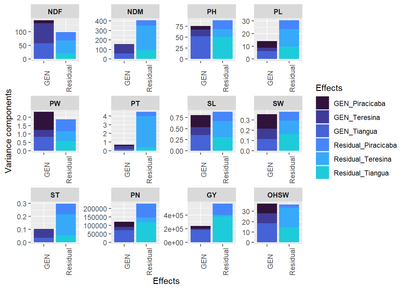

ggsave(plot=vcp,device = "pdf",filename ="Plots/varcomp.pdf",dpi = "retina",height = 6,width = 8)
ggsave(plot=vcp,device = "png",filename ="Plots/varcomp.png",dpi = "retina",height = 6,width = 8,bg = "white")

Broad-sense Heritability

custom_palette=viridis::turbo(n = 19)
her=do.call(rbind,herit)
colnames(her)

[1] "VAR" "h2"  "env"

heritp <- her |> 
  ggplot(aes(x = VAR, y = h2, fill = env)) + 
  geom_col(position = "stack", just = 0.5) + 
  theme(axis.text.x = element_text(angle = 90), 
        strip.text = element_text(face = "bold")) + 
  facet_wrap(~env, scales = "free") +
  labs(x = "Traits", y = "Broad-sense heritability", fill = "Environments") +
  scale_fill_manual(
    values = custom_palette)
heritp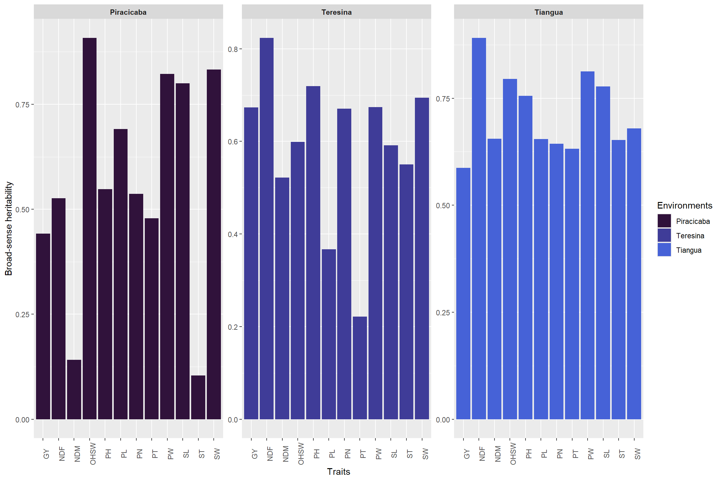

ggsave(plot=heritp,device = "pdf",filename ="Plots/herit.pdf",dpi = "retina",height = 6,width = 8)
ggsave(plot=heritp,device = "png",filename ="Plots/herit.png",dpi = "retina",height = 6,width = 8,bg = "white")

Mixed-effect models

mixedmodel <- gamem_met(LB,env = Env, gen = GEN, rep = Block,random = "gen" ,resp = everything())

Evaluating trait NDF |====                                       | 8% 00:00:00 
Evaluating trait NDM |=======                                    | 17% 00:00:00 
Evaluating trait PH |===========                                 | 25% 00:00:01

Evaluating trait PL |===============                             | 33% 00:00:01

Evaluating trait PW |==================                          | 42% 00:00:02

Evaluating trait PT |======================                      | 50% 00:00:02

Evaluating trait SL |==========================                  | 58% 00:00:02

Evaluating trait SW |=============================               | 67% 00:00:03

Evaluating trait ST |=================================           | 75% 00:00:03

Evaluating trait PN |=====================================       | 83% 00:00:04

Evaluating trait GY |========================================    | 92% 00:00:04

Evaluating trait OHSW |==========================================| 100% 00:00:05

---------------------------------------------------------------------------
P-values for Likelihood Ratio Test of the analyzed traits
---------------------------------------------------------------------------
    model      NDF    NDM       PH      PL       PW      PT       SL       SW
 COMPLETE       NA     NA       NA      NA       NA      NA       NA       NA
      GEN 3.43e-06 0.0788 4.83e-03 0.34753 3.70e-05 0.00102 8.53e-06 0.000199
  GEN:ENV 8.16e-06 0.0120 8.86e-06 0.00107 2.86e-05 1.00000 1.57e-02 0.000918
      ST       PN      GY     OHSW
      NA       NA      NA       NA
 0.00083 2.65e-01 0.21557 3.40e-07
 0.46110 5.04e-05 0.00108 3.51e-02
---------------------------------------------------------------------------
Variables with nonsignificant GxE interaction
PT ST 
---------------------------------------------------------------------------

library(dplyr)
library(tidyr)
library(purrr)

ne <- length(unique(LB$Env))
nr <- length(unique(LB$Block))

varcomp <- map_dfr(names(mixedmodel), function(tr){

  if(!"random" %in% names(mixedmodel[[tr]]))
    return(NULL)
  vc <- mixedmodel[[tr]]$random
  tibble(
    Trait = tr,
    sigma_g  = vc$Variance[vc$Group == "GEN"],
    sigma_ge = vc$Variance[vc$Group == "GEN:ENV"],
    sigma_e  = vc$Variance[vc$Group == "Residual"]
  )
})
genpar <- get_model_data(mixedmodel) %>%
  pivot_longer(
    cols = -Parameters,
    names_to = "Trait",
    values_to = "Value") %>%
  pivot_wider(
    names_from = Parameters,
    values_from = Value)

herit_table <- varcomp %>%
  left_join(genpar, by = "Trait") %>%
  dplyr::mutate(

    H2_individual =
      sigma_g /
      (sigma_g + sigma_ge + sigma_e),

    H2_MET =
      sigma_g /
      (sigma_g +
         sigma_ge/ne +
         sigma_e/(ne*nr)),

    H2mg_metan = h2mg) %>%
  dplyr::select(
    Trait,
    sigma_g,
    sigma_ge,
    sigma_e,
    H2_individual,
    H2_MET,
    H2mg_metan,
    Accuracy,
    GEIr2,
    rge,
    CVg,
    CVr,
    `CV ratio`)
herit_table

# A tibble: 12 × 13
   Trait    sigma_g    sigma_ge sigma_e H2_individual H2_MET H2mg_metan Accuracy
   <chr>      <dbl>       <dbl>   <dbl>         <dbl>  <dbl>      <dbl>    <dbl>
 1 NDF      38.9       16.9     3.41e+1        0.432   0.805      0.805    0.897
 2 NDM      25.5       35.7     1.54e+2        0.119   0.468      0.468    0.684
 3 PH       12.1       14.5     3.02e+1        0.213   0.597      0.597    0.772
 4 PL        0.947      3.51    1.08e+1        0.0620  0.286      0.286    0.534
 5 PW        0.423      0.273   6.15e-1        0.322   0.726      0.726    0.852
 6 PT        0.728      0       1.57e+0        0.316   0.806      0.806    0.898
 7 SL        0.199      0.0676  3.09e-1        0.346   0.778      0.778    0.882
 8 SW        0.0727     0.0430  1.32e-1        0.294   0.715      0.715    0.846
 9 ST        0.0376     0.00639 1.06e-1        0.250   0.729      0.729    0.854
10 PN     9271.     31235.      7.21e+4        0.0824  0.335      0.335    0.579
11 GY    22388.     58803.      1.81e+5        0.0853  0.360      0.360    0.600
12 OHSW     10.0        2.56    1.38e+1        0.379   0.807      0.807    0.898
# ℹ 5 more variables: GEIr2 <dbl>, rge <dbl>, CVg <dbl>, CVr <dbl>,
#   `CV ratio` <dbl>

Broad-sense Heritability MET

herit_met=get_model_data(mixedmodel, "h2")

custom_palette=viridis::turbo(n = 12)
heritp2 <- herit_met |> 
  ggplot(aes(x = VAR, y = h2, fill=VAR)) + 
  geom_col(position = "stack", just = 0.5) + 
  theme(axis.text.x = element_text(angle = 90), 
        strip.text = element_text(face = "bold")) +
  labs(x = "Traits", y = "Broad-sense heritability",fill = "Traits") +
  scale_fill_manual(
    values = custom_palette,  
  )
heritp2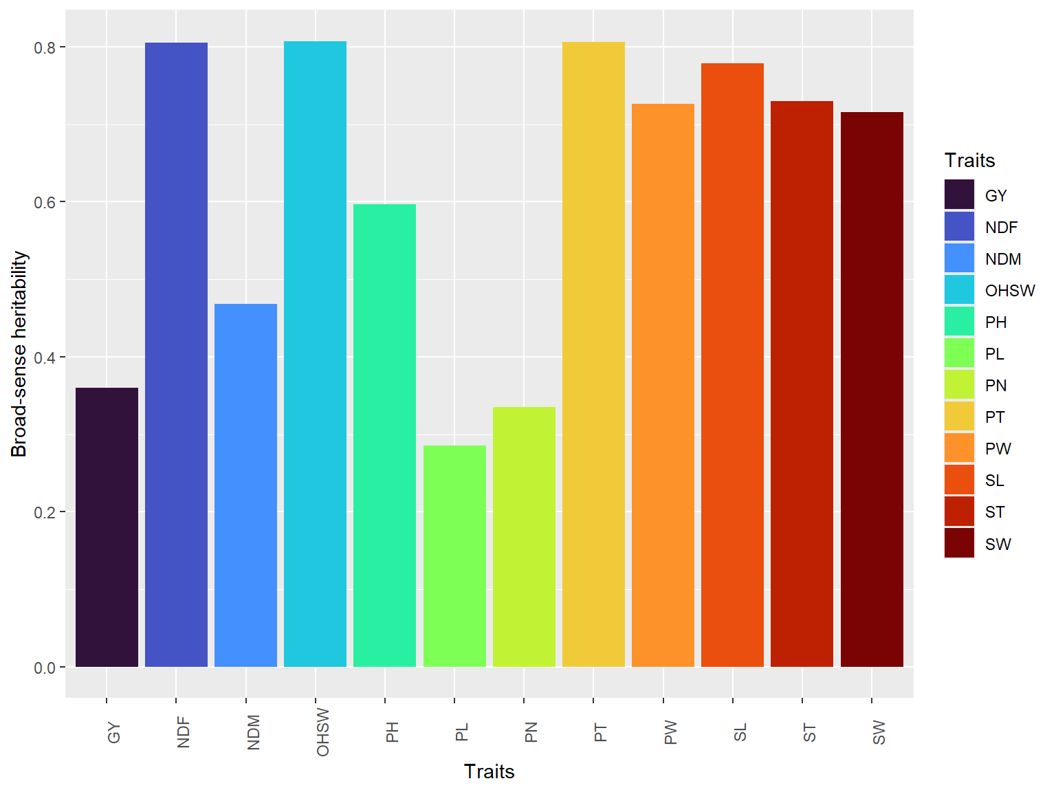

ggsave(plot=heritp2,device = "pdf",filename ="Plots/herit_met.pdf",dpi = "retina",height = 6,width = 8)
ggsave(plot=heritp2,device = "png",filename ="Plots/herit_met.png",dpi = "retina",height = 6,width = 8,bg = "white")

Culllis Heritability

traits <- c("PH", "NDF", "NDM", "OHSW", "PN", "GY")
library(sommer)
library(purrr)
library(dplyr)
calc_cullis <- function(tr){
  mod <- mmer(
    fixed  = as.formula(
      paste0(tr," ~ Env + Block:Env")
    ),
    random = ~ GEN + GEN:Env,
    rcov   = ~ units,
    data   = LB
  )
  vg <- mod$sigma$GEN
  C22 <- mod$PevU$GEN[[tr]]
  n_g <- nrow(C22)
  trC22 <- sum(diag(C22))

  av2 <- 2/n_g *
    (trC22 -
      (sum(C22)-trC22)/(n_g-1))

  H2 <- 1 - av2/(2*vg)

  tibble(
    Trait = tr,
    Cullis_H2 = as.numeric(H2))

}
Cullis_all <- map_dfr(
  traits,
  calc_cullis)

iteration    LogLik     wall    cpu(sec)   restrained
    1      -60.0291   15:30:50      0           0
    2      -57.008   15:30:50      0           0
    3      -56.1948   15:30:50      0           0
    4      -56.1213   15:30:50      0           0
    5      -56.1206   15:30:50      0           0

iteration    LogLik     wall    cpu(sec)   restrained
    1      -38.7664   15:30:50      0           0
    2      -26.3316   15:30:50      0           0
    3      -23.5492   15:30:50      0           0
    4      -23.3172   15:30:50      0           0
    5      -23.3144   15:30:50      0           0
    6      -23.3144   15:30:51      1           0

iteration    LogLik     wall    cpu(sec)   restrained
    1      -80.8335   15:30:51      0           0
    2      -80.7879   15:30:51      0           0
    3      -80.7715   15:30:51      0           0
    4      -80.7691   15:30:51      0           0
    5      -80.769   15:30:51      0           0

iteration    LogLik     wall    cpu(sec)   restrained
    1      -70.2583   15:30:51      0           0
    2      -64.6976   15:30:51      0           0
    3      -63.7078   15:30:51      0           0
    4      -63.6435   15:30:51      0           0
    5      -63.6432   15:30:51      0           0

iteration    LogLik     wall    cpu(sec)   restrained
    1      -76.0017   15:30:51      0           0
    2      -74.8831   15:30:51      0           0
    3      -74.5778   15:30:51      0           0
    4      -74.5462   15:30:52      1           0
    5      -74.5456   15:30:52      1           0

iteration    LogLik     wall    cpu(sec)   restrained
    1      -47.403   15:30:52      0           0
    2      -46.9832   15:30:52      0           0
    3      -46.8571   15:30:52      0           0
    4      -46.8422   15:30:52      0           0
    5      -46.8419   15:30:52      0           0

Cullis_all

# A tibble: 6 × 2
  Trait Cullis_H2
  <chr>     <dbl>
1 PH        0.528
2 NDF       0.752
3 NDM       0.403
4 OHSW      0.754
5 PN        0.281
6 GY        0.303

LRT

GYLRT = mixedmodel$GY$LRT
OHSWLRT = mixedmodel$OHSW$LRT 
NDFLRT = mixedmodel$NDF$LRT
NDMLRT = mixedmodel$NDM$LRT 
PHLRT = mixedmodel$PH$LRT
PNLRT = mixedmodel$PN$LRT
LRT = list(
  GY_LRT   = GYLRT,
  OHSW_LRT = OHSWLRT,
  NDF_LRT  = NDFLRT,
  NDM_LRT  = NDMLRT,
  PH_LRT   = PHLRT,
  PN_LRT   = PNLRT)
LRT

$GY_LRT
              model npar  logLik    AIC     LRT Df Pr(>Chisq)   
<none>            1   12 -2131.5 4286.9                         
(1 | GEN)         2   11 -2132.2 4286.5  1.5336  1   0.215571   
(1 | GEN:ENV)     3   11 -2136.8 4295.6 10.6932  1   0.001075 **
---
Signif. codes:  0 '***' 0.001 '**' 0.01 '*' 0.05 '.' 0.1 ' ' 1

$OHSW_LRT
              model npar  logLik    AIC    LRT Df Pr(>Chisq)    
<none>            1   12 -823.50 1671.0                         
(1 | GEN)         2   11 -836.50 1695.0 26.008  1    3.4e-07 ***
(1 | GEN:ENV)     3   11 -825.72 1673.4  4.441  1    0.03509 *  
---
Signif. codes:  0 '***' 0.001 '**' 0.01 '*' 0.05 '.' 0.1 ' ' 1

$NDF_LRT
              model npar  logLik    AIC    LRT Df Pr(>Chisq)    
<none>            1   12 -974.03 1972.1                         
(1 | GEN)         2   11 -984.81 1991.6 21.559  1  3.432e-06 ***
(1 | GEN:ENV)     3   11 -983.98 1990.0 19.900  1  8.159e-06 ***
---
Signif. codes:  0 '***' 0.001 '**' 0.01 '*' 0.05 '.' 0.1 ' ' 1

$NDM_LRT
              model npar  logLik    AIC    LRT Df Pr(>Chisq)  
<none>            1   12 -1148.4 2320.9                       
(1 | GEN)         2   11 -1150.0 2322.0 3.0888  1    0.07883 .
(1 | GEN:ENV)     3   11 -1151.6 2325.2 6.3046  1    0.01204 *
---
Signif. codes:  0 '***' 0.001 '**' 0.01 '*' 0.05 '.' 0.1 ' ' 1

$PH_LRT
              model npar  logLik    AIC     LRT Df Pr(>Chisq)    
<none>            1   12 -943.11 1910.2                          
(1 | GEN)         2   11 -947.08 1916.2  7.9428  1   0.004828 ** 
(1 | GEN:ENV)     3   11 -952.98 1928.0 19.7427  1   8.86e-06 ***
---
Signif. codes:  0 '***' 0.001 '**' 0.01 '*' 0.05 '.' 0.1 ' ' 1

$PN_LRT
              model npar  logLik    AIC     LRT Df Pr(>Chisq)    
<none>            1   12 -2009.8 4043.6                          
(1 | GEN)         2   11 -2010.4 4042.8  1.2403  1     0.2654    
(1 | GEN:ENV)     3   11 -2018.0 4058.0 16.4317  1  5.044e-05 ***
---
Signif. codes:  0 '***' 0.001 '**' 0.01 '*' 0.05 '.' 0.1 ' ' 1

write_xlsx(LRT, "LRT_LB.xlsx")

BLUPs

BLUPgen = list(
  GY_BLUP   = mixedmodel$GY$BLUPgen,
  OHSW_BLUP = mixedmodel$OHSW$BLUPgen,
  NDF_BLUP  = mixedmodel$NDF$BLUPgen,
  NDM_BLUP  = mixedmodel$NDM$BLUPgen,
  PH_BLUP   = mixedmodel$PH$BLUPgen,
  PN_BLUP   = mixedmodel$PN$BLUPgen)
head(BLUPgen)

$GY_BLUP
# A tibble: 40 × 7
    Rank GEN       Y BLUPg Predicted    LL    UL
   <dbl> <fct> <dbl> <dbl>     <dbl> <dbl> <dbl>
 1     1 L06   1380. 164.       913.  612. 1214.
 2     2 L32   1304. 144.       892.  591. 1193.
 3     3 L18   1113. 122.       871.  570. 1172.
 4     4 L24   1094. 115.       864.  563. 1165.
 5     5 L30   1085. 112.       861.  560. 1162.
 6     6 L07   1043.  96.8      846.  544. 1147.
 7     7 L17    893.  96.7      845.  544. 1146.
 8     8 L33    976.  72.7      821.  520. 1122.
 9     9 L05   1020.  66.2      815.  514. 1116.
10    10 L23    923.  53.5      802.  501. 1103.
# ℹ 30 more rows

$OHSW_BLUP
# A tibble: 40 × 7
    Rank GEN       Y BLUPg Predicted    LL    UL
   <dbl> <fct> <dbl> <dbl>     <dbl> <dbl> <dbl>
 1     1 L40    38.6  5.34      37.5  34.3  40.7
 2     2 L14    39.9  5.32      37.5  34.3  40.7
 3     3 L25    37.2  4.18      36.4  33.2  39.6
 4     4 L21    36.5  3.63      35.8  32.6  39.0
 5     5 L26    36.1  3.30      35.5  32.3  38.7
 6     6 L27    35.1  2.48      34.7  31.5  37.9
 7     7 L23    34.9  2.38      34.6  31.4  37.8
 8     8 L30    34.8  2.27      34.4  31.2  37.7
 9     9 L18    34.3  1.87      34.0  30.8  37.3
10    10 L20    34.2  1.79      34.0  30.8  37.2
# ℹ 30 more rows

$NDF_BLUP
# A tibble: 40 × 7
    Rank GEN       Y BLUPg Predicted    LL    UL
   <dbl> <fct> <dbl> <dbl>     <dbl> <dbl> <dbl>
 1     1 L23    55.3  9.73      53.3  47.0  59.7
 2     2 L28    55.3  9.73      53.3  47.0  59.7
 3     3 L16    51.6  6.69      50.3  43.9  56.7
 4     4 L26    51.2  6.42      50.0  43.7  56.4
 5     5 L30    51.1  6.33      49.9  43.6  56.3
 6     6 L19    50.8  6.06      49.7  43.3  56.0
 7     7 L22    50.4  5.79      49.4  43.0  55.8
 8     8 L27    50.3  5.70      49.3  43.0  55.7
 9     9 L18    50.1  5.52      49.1  42.8  55.5
10    10 L40    49.9  5.34      49.0  42.6  55.3
# ℹ 30 more rows

$NDM_BLUP
# A tibble: 40 × 7
    Rank GEN       Y BLUPg Predicted    LL    UL
   <dbl> <fct> <dbl> <dbl>     <dbl> <dbl> <dbl>
 1     1 L11   101    6.41      94.2  85.2 103. 
 2     2 L40   101.   5.70      93.5  84.4 103. 
 3     3 L23    98.9  4.87      92.6  83.6 102. 
 4     4 L28    98.3  4.61      92.4  83.4 101. 
 5     5 L19    97.6  4.25      92.0  83.0 101. 
 6     6 L25    96.1  3.57      91.3  82.3 100. 
 7     7 L16    95.9  3.47      91.2  82.2 100. 
 8     8 L18    95.6  3.31      91.1  82.1 100. 
 9     9 L22    94.8  2.95      90.7  81.7  99.8
10    10 L38    91.2  2.77      90.5  81.5  99.6
# ℹ 30 more rows

$PH_BLUP
# A tibble: 40 × 7
    Rank GEN       Y BLUPg Predicted    LL    UL
   <dbl> <fct> <dbl> <dbl>     <dbl> <dbl> <dbl>
 1     1 L25    59.9  9.28      52.9  47.6  58.2
 2     2 L28    52.0  4.53      48.1  42.8  53.4
 3     3 L22    50.0  3.37      47.0  41.7  52.3
 4     4 L30    48.5  2.43      46.0  40.7  51.3
 5     5 L23    48.4  2.40      46.0  40.7  51.3
 6     6 L27    48.2  2.26      45.9  40.6  51.1
 7     7 L26    48.2  2.25      45.8  40.6  51.1
 8     8 L18    47.5  1.88      45.5  40.2  50.8
 9     9 L19    47.0  1.59      45.2  39.9  50.5
10    10 L17    47.5  1.57      45.2  39.9  50.5
# ℹ 30 more rows

$PN_BLUP
# A tibble: 40 × 7
    Rank GEN       Y BLUPg Predicted    LL    UL
   <dbl> <fct> <dbl> <dbl>     <dbl> <dbl> <dbl>
 1     1 L32    963  104.       679.  480.  878.
 2     2 L05    847.  74.5      650.  451.  849.
 3     3 L04    844.  73.6      649.  450.  848.
 4     4 L02    832.  70.6      646.  447.  845.
 5     5 L07    812.  69.7      645.  446.  844.
 6     6 L33    803.  66.8      642.  443.  841.
 7     7 L24    775.  57.4      633.  434.  831.
 8     8 L17    744.  53.6      629.  430.  828.
 9     9 L30    739   45.3      620.  422.  819.
10    10 L18    734.  43.7      619.  420.  818.
# ℹ 30 more rows

write_xlsx(BLUPgen, "BLUPgen_LB.xlsx")

sommer_models <- setNames(
  map(traits, \(tr)
    mmer(
      fixed  = as.formula(
        paste0(tr, " ~ Env + Block:Env")
      ),
      random = ~ GEN + GEN:Env,
      rcov   = ~ units,
      data   = LB
    )
  ),
  traits)

iteration    LogLik     wall    cpu(sec)   restrained
    1      -60.0291   15:30:53      0           0
    2      -57.008   15:30:53      0           0
    3      -56.1948   15:30:53      0           0
    4      -56.1213   15:30:53      0           0
    5      -56.1206   15:30:53      0           0

iteration    LogLik     wall    cpu(sec)   restrained
    1      -38.7664   15:30:53      0           0
    2      -26.3316   15:30:53      0           0
    3      -23.5492   15:30:53      0           0
    4      -23.3172   15:30:53      0           0
    5      -23.3144   15:30:53      0           0
    6      -23.3144   15:30:53      0           0

iteration    LogLik     wall    cpu(sec)   restrained
    1      -80.8335   15:30:53      0           0
    2      -80.7879   15:30:53      0           0
    3      -80.7715   15:30:53      0           0
    4      -80.7691   15:30:53      0           0
    5      -80.769   15:30:54      1           0

iteration    LogLik     wall    cpu(sec)   restrained
    1      -70.2583   15:30:54      0           0
    2      -64.6976   15:30:54      0           0
    3      -63.7078   15:30:54      0           0
    4      -63.6435   15:30:54      0           0
    5      -63.6432   15:30:54      0           0

iteration    LogLik     wall    cpu(sec)   restrained
    1      -76.0017   15:30:54      0           0
    2      -74.8831   15:30:54      0           0
    3      -74.5778   15:30:54      0           0
    4      -74.5462   15:30:54      0           0
    5      -74.5456   15:30:54      0           0

iteration    LogLik     wall    cpu(sec)   restrained
    1      -47.403   15:30:54      0           0
    2      -46.9832   15:30:54      0           0
    3      -46.8571   15:30:54      0           0
    4      -46.8422   15:30:55      1           0
    5      -46.8419   15:30:55      1           0

sommer_blups <- map(
  traits,
  function(tr){

    data.frame(
      GEN = gsub("GEN", "", names(sommer_models[[tr]]$U$GEN[[tr]])),
      BLUP_sommer = as.numeric(
        sommer_models[[tr]]$U$GEN[[tr]]
      )
    )

  }
)
names(sommer_blups) <- traits

#Compare BLUPs- gamem_met and mmer 
library(dplyr)

compare_blups <- map_dfr(
  traits,
  function(tr){

    gamem_blup <-
      mixedmodel[[tr]]$BLUPgen |>
      dplyr::select(GEN, BLUPg)

    sommer_blup <- sommer_blups[[tr]]

    comp <- left_join(
      gamem_blup,
      sommer_blup,
      by = "GEN")
    tibble(
      Trait = tr,
      Correlation =
        cor(
          comp$BLUPg,
          comp$BLUP_sommer
        ),
      Max_Difference =
        max(
          abs(
            comp$BLUPg -
            comp$BLUP_sommer
          )
        )
    )

  }
)
compare_blups

# A tibble: 6 × 3
  Trait Correlation Max_Difference
  <chr>       <dbl>          <dbl>
1 PH          1.000      0.0000106
2 NDF         1.000      0.000226 
3 NDM         1.000      0.00106  
4 OHSW        1.000      0.0000478
5 PN          1.000      0.101    
6 GY          1.000      0.0933

library(dplyr)
library(tibble)

ebvMat <- data.frame(
  GEN = mixedmodel$GY$BLUPgen$GEN,
  GY   = mixedmodel$GY$BLUPgen$Predicted,
  OHSW = mixedmodel$OHSW$BLUPgen$Predicted,
  NDF  = mixedmodel$NDF$BLUPgen$Predicted,
  NDM  = mixedmodel$NDM$BLUPgen$Predicted,
  PH   = mixedmodel$PH$BLUPgen$Predicted,
  PN   = mixedmodel$PN$BLUPgen$Predicted
) |>
  column_to_rownames("GEN") |>
  as.matrix()
dim(ebvMat)

[1] 40  6

head(ebvMat)

          GY     OHSW      NDF      NDM       PH       PN
L06 913.1034 37.51991 53.34655 94.18319 52.87625 678.7407
L32 892.2353 37.49419 53.34655 93.47780 48.12310 649.6380
L18 870.6745 36.36019 50.30658 92.64571 46.96580 648.8006
L24 863.9895 35.80589 50.03834 92.38568 46.02591 645.7856
L30 860.5489 35.47762 49.94893 92.02164 45.99476 644.8933
L07 845.5058 34.66053 49.68070 91.34557 45.85358 641.9544

save(ebvMat,file = "Data/ebvMat.rda")

trait_units <- c(
  GY   = "kg/ha",   
  OHSW = "g",
  PH   = "cm",
  PN   = "number",
  NDF  = "number",
  NDM  = "number")
plot_trait_heatmap <- function(x, trait_name) {
  gen_order <- sprintf("L%02d", 1:40)
  df <- x[[trait_name]]$BLUPgen %>%
    filter(GEN %in% gen_order) %>%
    dplyr::mutate(
      GEN = factor(GEN, levels = gen_order),
      Trait = trait_name
    )
  ggplot(df, aes(x = GEN, y = Trait, fill = Predicted)) +
    geom_tile() +
    scale_fill_gradientn(
      colours = c("orange", "#E37383", "purple"),
      name = bquote(hat(y)~"("~.(trait_units[[trait_name]])~")")) +
    labs(x = NULL, y = NULL) +
    theme_minimal(base_size = 14) +
    theme(
      axis.text.x = element_text(angle = 90, vjust = 0.5, hjust = 1, face = "bold"),
      axis.text.y = element_text(angle = 90, face = "bold"),
      legend.position = "right",
      panel.grid = element_blank())
}
traits <- c("GY", "OHSW", "PH", "PN", "NDF", "NDM")
BLUP_heatmaps <- lapply(traits, function(trait) {
  plot_trait_heatmap(mixedmodel, trait)
})
library(ggpubr)
blups_heatmap_panel <- ggarrange(
  plotlist = BLUP_heatmaps,
  ncol = 2, nrow = 3,
  labels = c("A", "B", "C", "D", "E", "F"), font.label = list(size = 10, face = "bold"),
  align = "v")
ggsave(
  "BLUPs_LB.pdf",
  blups_heatmap_panel,
  width = 14,
  height = 12,
  dpi = 600)

trait_units <- c(
  GY   = "kg/ha",   
  OHSW = "g",
  PH   = "cm",
  PN   = "number",
  NDF  = "number",
  NDM  = "number")
plot_trait_dot <- function(x, trait_name){
  gen_order <- sprintf("L%02d", 1:40)
  df <- x[[trait_name]]$BLUPgen %>%
    filter(GEN %in% gen_order) %>%
    dplyr::mutate(
      GEN = factor(GEN, levels = gen_order),
      Trait = trait_name)
  ggplot(df, aes(x = Trait, y = GEN)) +
    geom_point(
      aes(
        size  = round(abs(Predicted)),
        color = Predicted),
      alpha = 0.75) +
    scale_color_gradientn(
      colours = c("orange", "lightpink", "purple"),
      name = bquote(hat(y)~"("~.(trait_units[[trait_name]])~")"),
      guide = guide_colorbar(
    barheight = unit(0.3, "cm"),
    barwidth = unit(4, "cm"))) +

    scale_size(range = c(8,11), guide = "none") +

    labs(
      x = NULL,
      y = NULL) +

    theme_linedraw(base_size = 12) +
    theme(
      axis.text.x = element_text(
        angle = 0,
        hjust = 1,
        vjust = 1,
        face = "bold"),
      axis.text.y = element_text(face = "bold"),
      panel.grid = element_blank(),
      legend.position = "bottom",legend.title.position = "bottom",
      legend.text = element_text(size = 7.5, face = "bold"),
      legend.title = element_text(size = 8, face = "bold"))
}
traits <- c("GY", "OHSW", "PN", "PH", "NDF", "NDM")

BLUP_dots <- lapply(traits, function(tr){
  plot_trait_dot(mixedmodel, tr)
})

library(ggpubr)
#BLUP_dots

blups_d_panel <- ggarrange(
  plotlist = BLUP_dots,
  ncol = 6, nrow = 1,
  labels = c("A", "B", "C", "D", "E", "F"), vjust = 0.11,
  font.label = list(face = "bold"),label.y = 0.01,
  align = "v")
blups_d_panel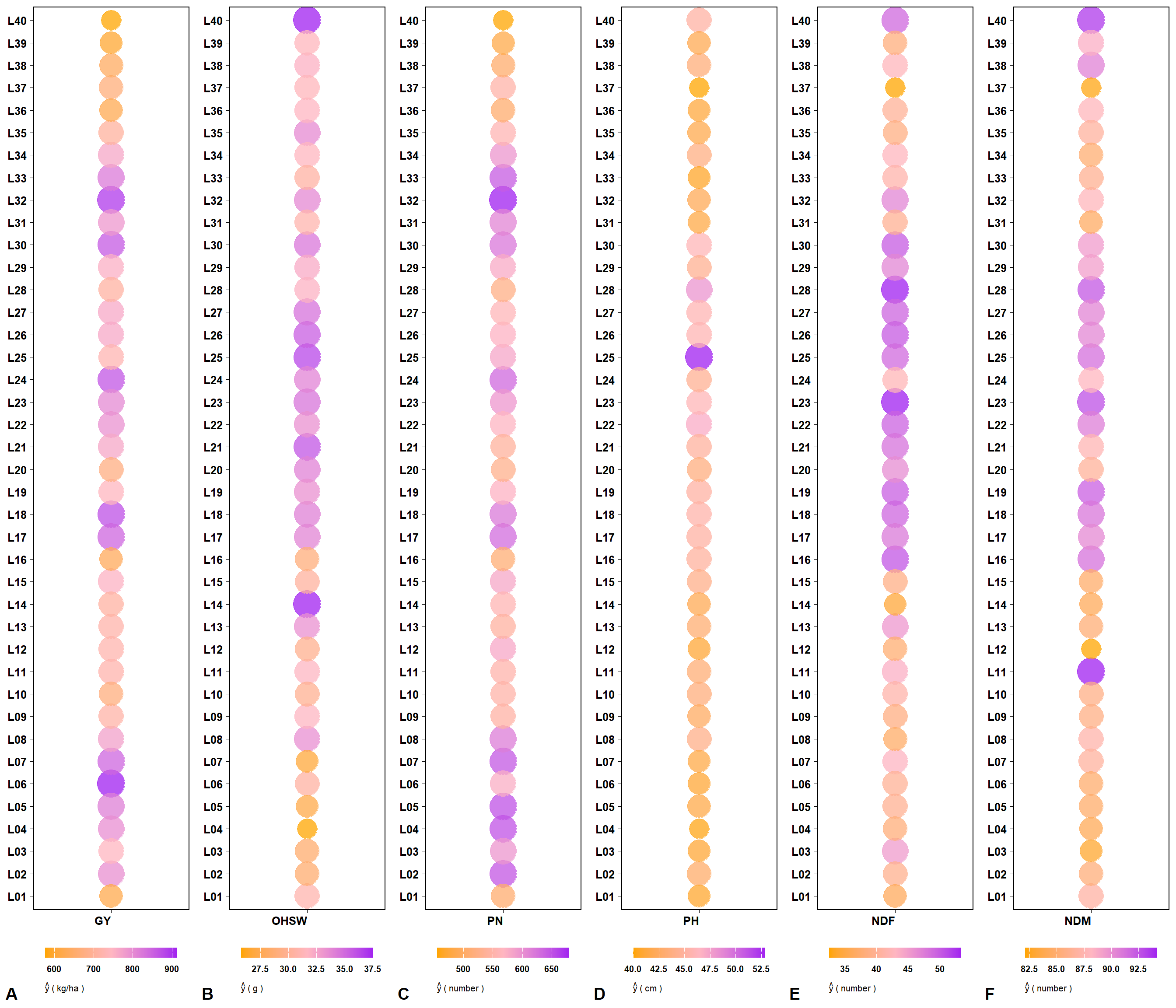

ggsave(
  "BLUPs_d2_LB.pdf",
  blups_d_panel, height = 11, width = 13,
  dpi = 600)

Correlation

corrplot = plot(
  corr_coef(LB, NDF, NDM, PH, PN, GY, OHSW),
  type = "upper",
  diag = FALSE,
  reorder = T,
  signif = c("stars", "pval"),
  show = c("all", "signif"),
  p_val = 0.05,
  caption = TRUE,
  digits.cor = 2,
  digits.pval = 3,
  col.low = "orange",
  col.mid = "white",
  col.high = "purple",
  lab.x.position = "top",
  lab.y.position = "left",   
  legend.position = "right",
  legend.title = "Pearson's\nCorrelation",
  size.text.cor = 5,
  size.text.signif = 5,
  size.text.lab = 14)

ggsave("Correlation.pdf",corrplot, width = 7, height = 6, dpi = 600)

library(circlize)
# Correlation matrix
corr_mat <- matrix(
  c(
    1.000, 0.587, 0.205,-0.230,-0.264,-0.129,
    0.587, 1.000, 0.224,-0.214,-0.262,-0.131,
    0.205, 0.224, 1.000, 0.160, 0.177, 0.413,
   -0.230,-0.214, 0.160, 1.000, 0.861, 0.123,
   -0.264,-0.262, 0.177, 0.861, 1.000, 0.267,
   -0.129,-0.131, 0.413, 0.123, 0.267, 1.000),
  nrow = 6,
  byrow = TRUE)
traits <- c(
  "NDF",
  "NDM",
  "PH",
  "PN",
  "GY",
  "OHSW")
rownames(corr_mat) <- traits
colnames(corr_mat) <- traits
# Convert matrix to links
corr_df <- data.frame()
for(i in 1:(nrow(corr_mat)-1)){
  for(j in (i+1):ncol(corr_mat)){
    corr_df <- rbind(
      corr_df,
      data.frame(
        from  = rownames(corr_mat)[i],
        to    = colnames(corr_mat)[j],
        value = corr_mat[i,j]))
  }
}
# Link colors
corr_df$link_col <- ifelse(
  corr_df$value > 0,
  "purple",
  "orange")
# Trait colors
grid_cols <- c(
  NDF  = "grey60",
  NDM  = "grey40",
  PH   = "grey60",
  PN   = "grey40",
  GY   = "grey60",
  OHSW = "grey40")
# Plot
circos.clear()
chordDiagram(
  x = corr_df[, c("from","to","value")],
  grid.col = grid_cols,
  col = corr_df$link_col,
  transparency = 0.80,
  directional = 0,
  # MUCH THINNER LINES
  link.lwd = 0.5 + abs(corr_df$value) * 2,
  annotationTrack = "grid",
  preAllocateTracks = list(
    track.height = 0.12))
# Trait labels
circos.track(
  track.index = 1,
  panel.fun = function(x,y){
    circos.text(
      CELL_META$xcenter,
      CELL_META$ylim[1],
      CELL_META$sector.index,
      facing = "clockwise",
      niceFacing = TRUE,
      adj = c(0,0.5),
      font = 2,
      cex = 1.3)
  },
  bg.border = NA
)
# Title
title(
  "Pearson Correlation Network",
  font.main = 2,
  cex.main = 1.4)
# Legends
legend(
  "topleft",
  legend = c(
    "Positive",
    "Negative"),
  col = c(
    "purple",
    "orange"),
  lwd = 4,
  title = "Correlation sign",
  bty = "n",
  cex = 1)
legend(
  "topright",
  legend = c(
    "|r| = 0.2",
    "|r| = 0.5",
    "|r| = 0.8"),
  lwd = c(
    0.5 + 0.2*2,
    0.5 + 0.5*2,
    0.5 + 0.8*2),
  col = "black",
  title = "Correlation strength",
  bty = "n",
  cex = 1)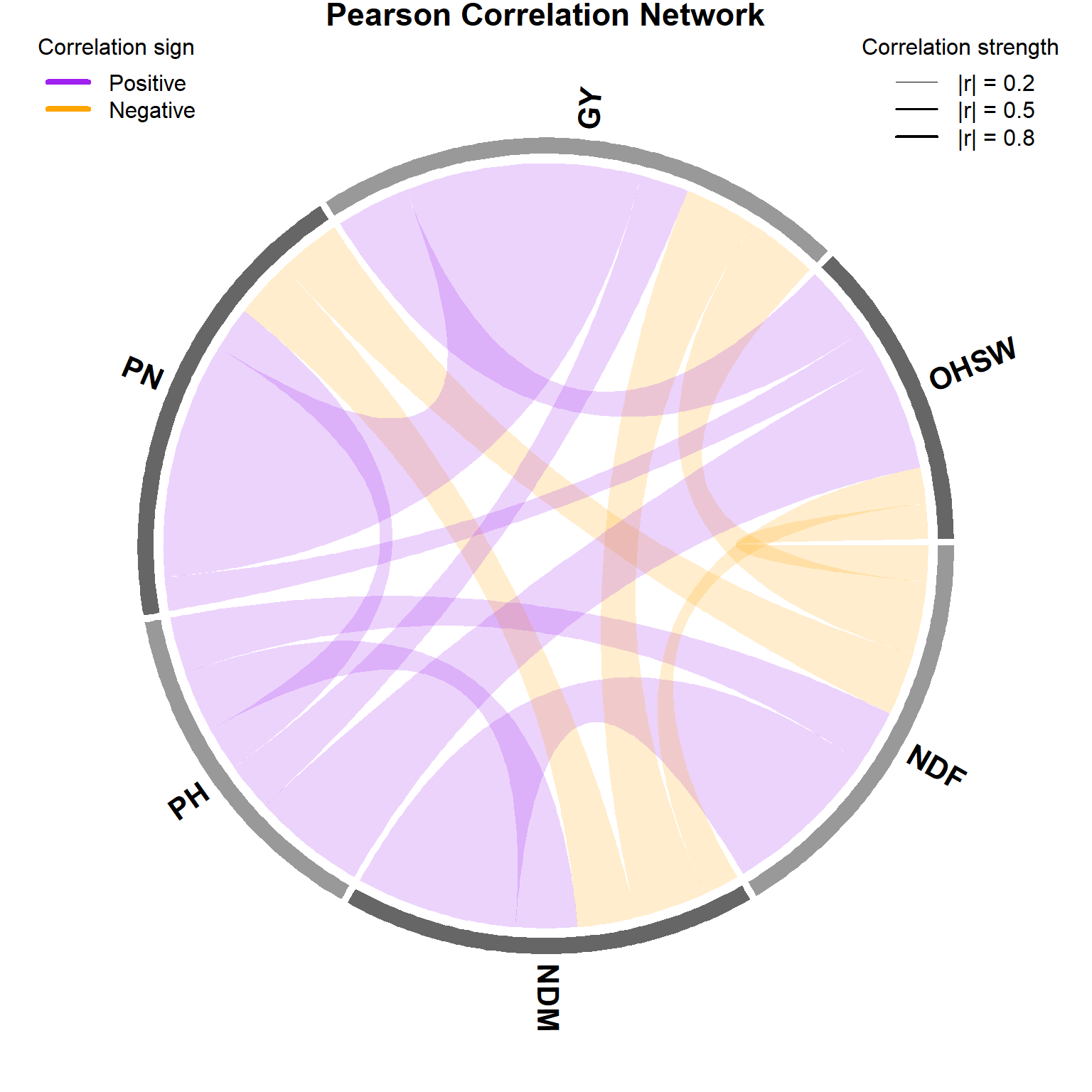

pdf(
  "Correlation_Chord_Diagram.pdf",
  width = 8,
  height = 8)
dev.off()

GGE BIPLOT

Which-Won-where

www <- list()

for(tr in traits){
  gge3_tr <- gge(LB, Env, GEN, resp = tr, svp = "symmetrical")
  
  p <- plot(gge3_tr,
            type = 3,
            col.env = "orange",
            col.gen = "purple",
            shape.gen = 21,
            shape.env = 23,
            col.alpha = 0.3,
            arrow.color = "purple",
            size.text.gen = 4,
            size.text.win = 8,
            size.text.env = 8,
            size.shape = 5,
            size.shape.win = 10,
            large_label = 10,
            repel = TRUE,
            max_overlaps = 40, 
            repulsion =8,
            col.line = "orange",
            plot_theme = theme_metan_minimal())
  
  p_try <- try({
    p2 <- p + labs(title = tr, subtitle = NULL) +
            theme(plot.title = element_text(hjust = 0.5, face = "bold"))
    p <- p2
    NULL
  }, silent = TRUE)
  
  if(inherits(p_try, "try-error") || !inherits(p, "ggplot")) {
    p_grob <- ggpubr::as_ggplot(p)            
    p <- p_grob + labs(title = tr, subtitle = NULL) +
              theme(plot.title = element_text(hjust = 0.5, face = "bold"))
  }
  
  www[[tr]] <- p
}
www_lb <- ggarrange(
  www[["GY"]],  www[["OHSW"]], www[["PN"]],
  www[["PH"]],  www[["NDF"]],  www[["NDM"]],
  ncol = 2, nrow = 3,
  common.legend = TRUE, legend = "bottom",
  labels = c("A","B","C","D","E","F"),
  font.label = list(size = 12, face = "bold"),
  align = "hv",
  hjust = -0.5,
  vjust = 1.5)
www_lb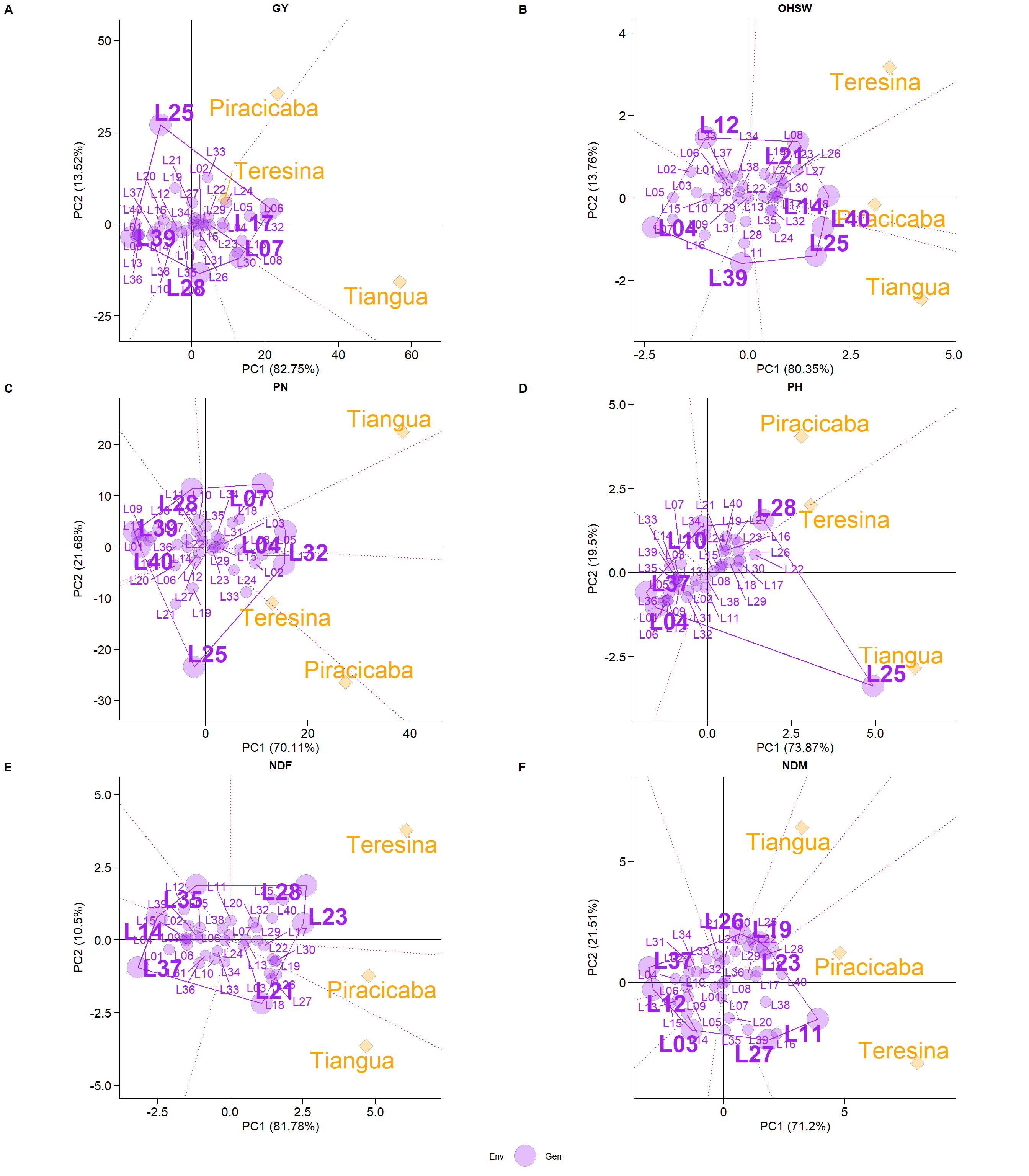

ggsave("Which-won-Where2.pdf", www_lb,width = 14, height = 16, dpi = 600)

Mean_performance vs. stability

dir.create("Mean_performance_vs_stability", showWarnings = FALSE)

mps_list <- list()

for(tr in traits){
    gge2_tr <- gge(
    LB,
    Env,
    GEN,
    resp = tr,
    svp = "genotype")
  # Plot type 2
  p <- plot(gge2_tr,
            type = 2,
            col.env = "orange",
            col.gen = "purple",
            shape.gen = 21,
            shape.env = 23,
            col.alpha = 0.3,
            arrow.color = "purple",
            size.text.gen = 4,
            size.text.env = 5,
            size.shape = 5,
            large_label = 1,
            repel = TRUE,
            max_overlaps = 10, 
            repulsion =40,
            col.line = "orange",
            axis_expand = 1.2,
            plot_theme = theme_metan_minimal())
  
  p_try <- try({
    p2 <- p + labs(title = tr, subtitle = NULL) +
      theme(plot.title = element_text(hjust = 0.5, face = "bold"))
    p <- p2
    NULL
  }, silent = TRUE)
  
  if(inherits(p_try, "try-error") || !inherits(p, "ggplot")) {
    p_grob <- ggpubr::as_ggplot(p)
    p <- p_grob + labs(title = tr, subtitle = NULL) +
      theme(plot.title = element_text(hjust = 0.5, face = "bold"))
  }
  
  mps_list[[tr]] <- p2}

mps_panel <- ggarrange(
  mps_list[["GY"]],  mps_list[["OHSW"]], mps_list[["PN"]],
  mps_list[["PH"]],  mps_list[["NDF"]],  mps_list[["NDM"]],
  ncol = 2, nrow = 3,
  common.legend = TRUE, legend = "bottom",
  labels = c("A","B","C","D","E","F"),
  font.label = list(size = 10, face = "bold"),
  align = "hv")
mps_panel = annotate_figure(
  mps_panel,
  top = text_grob("", size = 14),
  fig.lab = "",
  fig.lab.pos = "bottom")

mps_GY <- gge(
  LB,
  Env,
  GEN,
  resp = "GY",
  svp = "genotype")

mpsp_GY <- plot(
  mps_GY,
  type = 2,
  col.env = "orange",
  col.gen = "purple",
  col.line = "grey50",
  size.text.gen = 4,
  size.text.env = 5,
  repel = TRUE,
  repulsion = 0,
  max_overlaps = 40,
  axis_expand = 1.1,
  plot_theme = theme_classic(base_size = 12)) +
  labs(title = NULL, subtitle = NULL)

mpsp_OHSW <- gge(
  LB,
  Env,
  GEN,
  resp = "OHSW",
  svp = "genotype")

mpspp_OHSW <- plot(
  mpsp_OHSW,
  type = 2,
  col.env = "orange",
  col.gen = "purple",
  col.line = "grey50",
  size.text.gen = 4,
  size.text.env = 5,
  repel = TRUE,
  repulsion = 20,
  max_overlaps = 30,
  axis_expand = 1.08,
  plot_theme = theme_classic(base_size = 14)) +
  labs(title = NULL, subtitle = NULL)

mpsp_PN <- gge(
  LB,
  Env,
  GEN,
  resp = "PN",
  svp = "genotype")

mpspp_PN <- plot(
  mpsp_PN,
  type = 2,
  col.env = "orange",
  col.gen = "purple",
  col.line = "grey50",
  size.text.gen = 4,
  size.text.env = 5,
  repel = TRUE,
  repulsion = 20,
  max_overlaps = 30,
  axis_expand = 1.1,
  plot_theme = theme_classic(base_size = 14)) +
  labs(title = NULL, subtitle = NULL)

mpsp_PH <- gge(
  LB,
  Env,
  GEN,
  resp = "PH",
  svp = "genotype")

mpspp_PH <- plot(
  mpsp_PH,
  type = 2,
  col.env = "orange",
  col.gen = "purple",
  col.line = "grey50",
  size.text.gen = 4,
  size.text.env = 5,
  repel = TRUE,
  repulsion = 20,
  max_overlaps = 30,
  axis_expand = 1.05,
  plot_theme = theme_classic(base_size = 14)) +
  labs(title = NULL, subtitle = NULL)

mpsp_NDF <- gge(
  LB,
  Env,
  GEN,
  resp = "NDF",
  svp = "genotype")

mpspp_NDF <- plot(
  mpsp_NDF,
  type = 2,
  col.env = "orange",
  col.gen = "purple",
  col.line = "grey50",
  size.text.gen = 4,
  size.text.env = 5,
  repel = TRUE,
  repulsion = 20,
  max_overlaps = 30,
  axis_expand = 1.1,
  plot_theme = theme_classic(base_size = 14)) +
  labs(title = NULL, subtitle = NULL)

mpsp_NDM <- gge(
  LB,
  Env,
  GEN,
  resp = "NDM",
  svp = "genotype")

mpspp_NDM <- plot(
  mpsp_NDM,
  type = 2,
  col.env = "orange",
  col.gen = "purple",
  col.line = "grey50",
  size.text.gen = 4,
  size.text.env = 5,
  repel = TRUE,
  repulsion = 20,
  max_overlaps = 30,
  axis_expand = 1.07,
  plot_theme = theme_classic(base_size = 14)) +
  labs(title = NULL, subtitle = NULL)

mpsp_GY <- mpsp_GY +
  ggtitle("GY") +
  theme(plot.title = element_text(hjust = 0.5, face = "bold"))

mpspp_OHSW <- mpspp_OHSW +
  ggtitle("OHSW") +
  theme(plot.title = element_text(hjust = 0.5, face = "bold"))

mpspp_PN <- mpspp_PN +
  ggtitle("PN") +
  theme(plot.title = element_text(hjust = 0.5, face = "bold"))

mpspp_PH <- mpspp_PH +
  ggtitle("PH") +
  theme(plot.title = element_text(hjust = 0.5, face = "bold"))

mpspp_NDF <- mpspp_NDF +
  ggtitle("NDF") +
  theme(plot.title = element_text(hjust = 0.5, face = "bold"))

mpspp_NDM <- mpspp_NDM +
  ggtitle("NDM") +
  theme(plot.title = element_text(hjust = 0.5, face = "bold"))

common_theme <- theme(
  legend.position = "bottom",
  panel.grid = element_blank(),
  plot.title = element_text(
    hjust = 0.5,
    face = "bold",
    size = 12
  )
)
mpsp_GY     <- mpsp_GY + common_theme
mpspp_OHSW  <- mpspp_OHSW + common_theme
mpspp_PN    <- mpspp_PN + common_theme
mpspp_PH    <- mpspp_PH + common_theme
mpspp_NDF   <- mpspp_NDF + common_theme
mpspp_NDM   <- mpspp_NDM + common_theme
mps_panel <- ggarrange(
  mpsp_GY,
  mpspp_OHSW,
  mpspp_PN,
  mpspp_PH,
  mpspp_NDF,
  mpspp_NDM,
  ncol = 2,
  nrow = 3,
  common.legend = TRUE,
  legend = "bottom",
  labels = c("A","B","C","D","E","F"),
  font.label = list(
    size = 12,
    face = "bold"
  )
)
mps_panel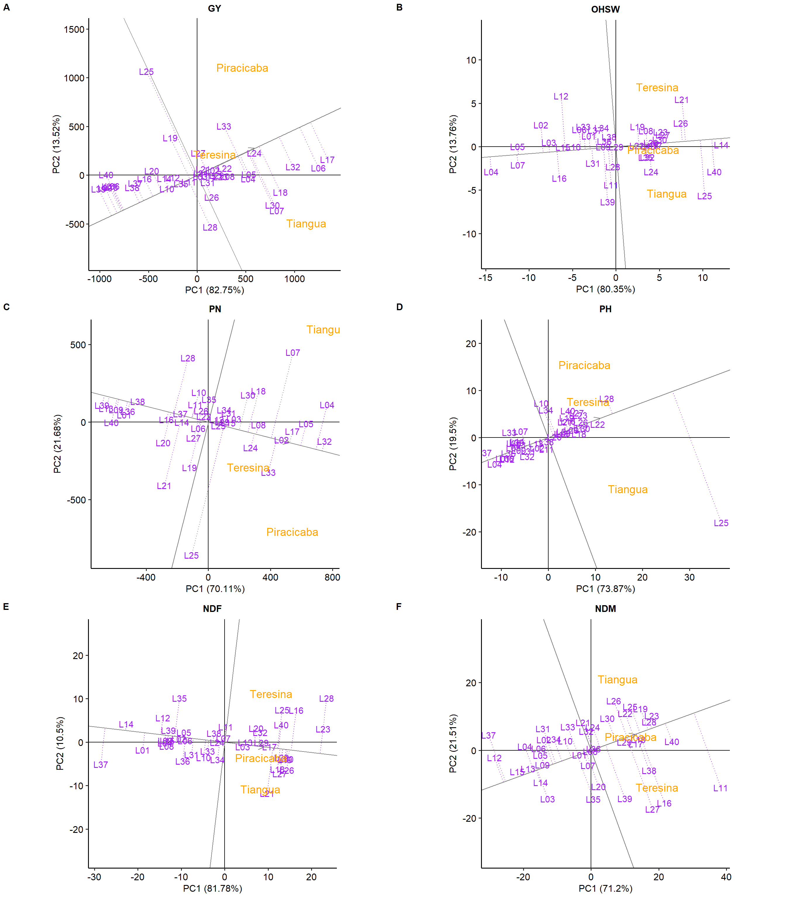

ggsave("Mean Performance vs Stability_LB2.pdf", mps_panel, width = 14, height = 16, dpi = 600)

Discriminativeness vs. representativeness

library(ggplot2)
library(ggpubr)

dir.create("Discriminativeness_vs_Representativeness", showWarnings = FALSE)

dr_list <- list()

for(tr in traits){

  gge4_tr <- gge(
    LB,
    Env,
    GEN,
    resp = tr,
    centering = "environment",
    scaling = "none",
    svp = "environment"
  )
  
  p4 <- plot(gge4_tr,
             type = 4,
             col.env = "orange",
             col.gen = "purple",
             size.text.gen = 4,
             size.text.env = 4 ,
             repel = TRUE,
             repulsion = 10,
             col.line = "orange",
             size.line = 0.5,
             col.circle = "grey",
             col.alpha = 0.4,
             max_overlaps = 20,
             plot_theme = theme_metan_minimal())
  p_try <- try({
    p4_mod <- p4 +
      labs(title = tr, subtitle = NULL) +
      theme(plot.title = element_text(hjust = 0.5, face = "bold"))
    p4 <- p4_mod
    NULL
  }, silent = TRUE)
  if(inherits(p_try, "try-error") || !inherits(p4, "ggplot")) {
    p_grob <- ggpubr::as_ggplot(p4)
    p4 <- p_grob +
      labs(title = tr, subtitle = NULL) +
      theme(plot.title = element_text(hjust = 0.5, face = "bold"))
  }
  dr_list[[tr]] <- p4
}
dr_panel <- ggarrange(
  dr_list[["GY"]],  dr_list[["OHSW"]], dr_list[["PN"]],
  dr_list[["PH"]],  dr_list[["NDF"]],  dr_list[["NDM"]],
  ncol = 2, nrow = 3,
  common.legend = TRUE, legend = "bottom",
  labels = c("A","B","C","D","E","F"),
  font.label = list(size = 10, face = "bold"), 
  align = "hv",
  hjust = -0.5,
  vjust = 1.5
)
dr_panel = annotate_figure(
  dr_panel,
  top = text_grob("", size = 14),
  fig.lab = "",
  fig.lab.pos = "bottom"
)

dr_GY <- gge(
  LB,
  Env,
  GEN,
  resp = "GY",
  centering = "environment",
  scaling = "none",
  svp = "environment"
)

drp_GY <- plot(
  dr_GY,
  type = 4,
  col.env = "orange",
  col.gen = "purple",
  size.text.gen = 3,
  size.text.env = 5,
  col.alpha = 0.2,
  repel = TRUE,
  repulsion = 5,
  max_overlaps = 20,
  col.line = "darkorange",
  plot_theme = theme_classic(base_size = 12)
) +
  labs(title = NULL, subtitle = NULL)

dr_OHSW <- gge(
  LB,
  Env,
  GEN,
  resp = "OHSW",
  centering = "environment",
  scaling = "none",
  svp = "environment"
)

drp_OHSW <- plot(
  dr_OHSW,
  type = 4,
  col.env = "orange",
  col.gen = "purple",
  size.text.gen = 3,
  size.text.env = 5,
  col.alpha = 0.2,
  repel = TRUE,
  repulsion = 5,
  max_overlaps = 20,
  col.line = "darkorange",
  plot_theme = theme_classic(base_size = 12)
) +
  labs(title = NULL, subtitle = NULL)

dr_PN <- gge(
  LB,
  Env,
  GEN,
  resp = "PN",
  centering = "environment",
  scaling = "none",
  svp = "environment"
)

drp_PN <- plot(
  dr_PN,
  type = 4,
  col.env = "orange",
  col.gen = "purple",
  size.text.gen = 3,
  size.text.env = 5,
  col.alpha = 0.2,
  repel = TRUE,
  repulsion = 5,
  max_overlaps = 10,
  col.line = "darkorange",
  plot_theme = theme_classic(base_size = 12)
) +
  labs(title = NULL, subtitle = NULL)

dr_PH<- gge(
  LB,
  Env,
  GEN,
  resp = "PH",
  centering = "environment",
  scaling = "none",
  svp = "environment"
)

drp_PH <- plot(
  dr_PH,
  type = 4,
  col.env = "orange",
  col.gen = "purple",
  size.text.gen = 3,
  size.text.env = 5,
  col.alpha = 0.2,
  repel = TRUE,
  repulsion = 5,
  max_overlaps = 20,
  col.line = "darkorange",
  plot_theme = theme_classic(base_size = 12)
) +
  labs(title = NULL, subtitle = NULL)

dr_NDF<- gge(
  LB,
  Env,
  GEN,
  resp = "NDF",
  centering = "environment",
  scaling = "none",
  svp = "environment"
)

drp_NDF <- plot(
  dr_NDF,
  type = 4,
  col.env = "orange",
  col.gen = "purple",
  size.text.gen = 3,
  size.text.env = 5,
  col.alpha = 0.2,
  repel = TRUE,
  repulsion = 5,
  max_overlaps = 20,
  col.line = "darkorange",
  plot_theme = theme_classic(base_size = 12)
) +
  labs(title = NULL, subtitle = NULL)

dr_NDM<- gge(
  LB,
  Env,
  GEN,
  resp = "NDM",
  centering = "environment",
  scaling = "none",
  svp = "environment"
)

drp_NDM <- plot(
  dr_NDM,
  type = 4,
  col.env = "orange",
  col.gen = "purple",
  size.text.gen = 3,
  size.text.env = 5,
  col.alpha = 0.2,
  repel = TRUE,
  repulsion = 5,
  max_overlaps = 10,
  col.line = "darkorange",
  plot_theme = theme_classic(base_size = 12)
) +
  labs(title = NULL, subtitle = NULL)

drp_GY <- drp_GY +
  ggtitle("GY") +
  theme(plot.title = element_text(hjust = 0.5, face = "bold"))

drp_OHSW <- drp_OHSW +
  ggtitle("OHSW") +
  theme(plot.title = element_text(hjust = 0.5, face = "bold"))

drp_PN <- drp_PN +
  ggtitle("PN") +
  theme(plot.title = element_text(hjust = 0.5, face = "bold"))

drp_PH <- drp_PH +
  ggtitle("PH") +
  theme(plot.title = element_text(hjust = 0.5, face = "bold"))

drp_NDF <- drp_NDF +
  ggtitle("NDF") +
  theme(plot.title = element_text(hjust = 0.5, face = "bold"))

drp_NDM <- drp_NDM +
  ggtitle("NDM") +
  theme(plot.title = element_text(hjust = 0.5, face = "bold"))
common_theme <- theme(
  legend.position = "bottom",
  panel.grid = element_blank(),
  plot.title = element_text(
    hjust = 0.5,
    face = "bold",
    size = 12))
drp_GY    <- drp_GY    + common_theme
drp_OHSW  <- drp_OHSW  + common_theme
drp_PN    <- drp_PN    + common_theme
drp_PH    <- drp_PH    + common_theme
drp_NDF   <- drp_NDF   + common_theme
drp_NDM   <- drp_NDM   + common_theme
dr_panel <- ggarrange(
  drp_GY,
  drp_OHSW,
  drp_PN,
  drp_PH,
  drp_NDF,
  drp_NDM,
  ncol = 2,
  nrow = 3,
  common.legend = TRUE,
  legend = "bottom",
  labels = c("A","B","C","D","E","F"),
  font.label = list(
    size = 12,
    face = "bold"
  )
)
dr_panel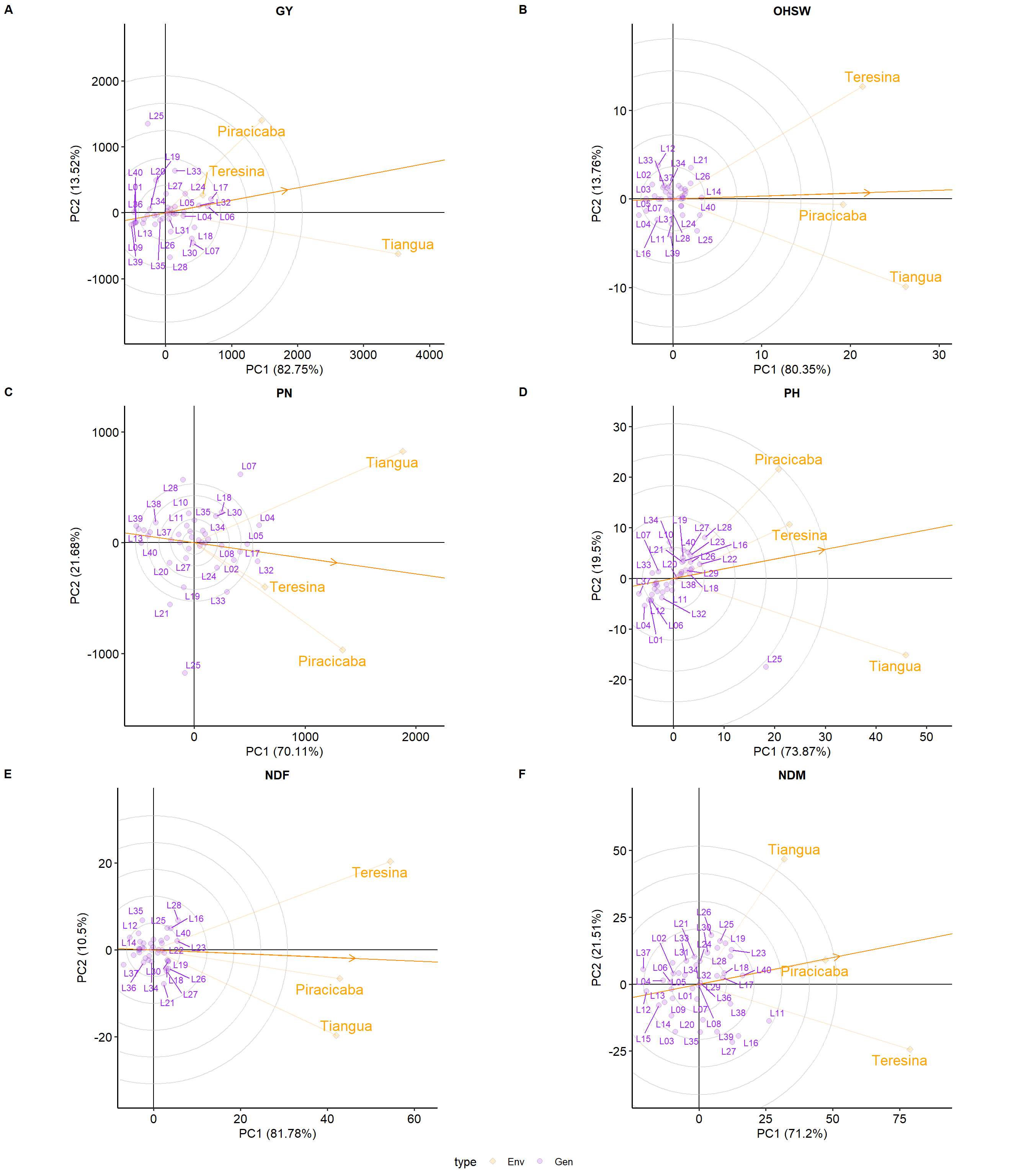

ggsave("Discriminativeness vs Representativeness_LB.pdf", dr_panel, width = 14, height = 16, dpi = 600)

Simultaneous Selection

Desire Gain Index

# DESIRE INDEX FUNCTION
gainDiff <- function(ebvMat, b_ebv, dGain, nSel){ 
  take <- order(ebvMat %*% b_ebv, decreasing = TRUE)[1:nSel]
  mu_Sel <- colMeans(ebvMat[take, ])
  resp   <- mu_Sel - colMeans(ebvMat)
  resp   <- resp / sqrt(sum(resp^2))
  sum((resp - dGain)^2)
}

ebvMat <- ebvMat[complete.cases(ebvMat), ]
#COV MATRIX -EBVS
library(AlphaSimR)

Warning: pacote 'AlphaSimR' foi compilado no R versão 4.4.3

Carregando pacotes exigidos: R6


Anexando pacote: 'AlphaSimR'

O seguinte objeto é mascarado por 'package:ggpubr':

    mutate

O seguinte objeto é mascarado por 'package:metan':

    mutate

O seguinte objeto é mascarado por 'package:dplyr':

    mutate

(G_ebv <- AlphaSimR::popVar(ebvMat))

          [,1]       [,2]      [,3]       [,4]       [,5]      [,6]
[1,] 6619.9044 218.241188 423.56486 252.987379 189.859236 4066.9162
[2,]  218.2412   7.357991  14.14453   8.392790   6.275343  134.1794
[3,]  423.5649  14.144528  28.50691  16.749936  12.432327  263.6634
[4,]  252.9874   8.392790  16.74994  10.010313   7.477405  156.8425
[5,]  189.8592   6.275343  12.43233   7.477405   6.242205  117.3492
[6,] 4066.9162 134.179444 263.66338 156.842455 117.349159 2535.0429

#desired gains
desiredGain <- c(
  GY   =  2,
  OHSW =  1,
  NDF  = -1,
  NDM  = -1,
  PH   =  0,
  PN   =  1
)
desiredGain <- desiredGain / sqrt(sum(desiredGain^2))
sum(desiredGain^2)

[1] 1

b_ebv <- solve(G_ebv) %*% desiredGain

nSel <- 5
opt <- optim(
  par     = b_ebv,
  fn      = gainDiff,
  ebvMat  = ebvMat,
  dGain   = desiredGain,
  nSel    = nSel
)
(opt_weights <- opt$par)

            [,1]
[1,] -0.06221013
[2,]  2.68757780
[3,] -0.13848027
[4,] -1.84924576
[5,]  0.42431249
[6,]  0.06686236

DesireIndex <- ebvMat %*% opt_weights
DesireIndex <- data.frame(
  GEN = rownames(ebvMat),
  DesireIndex = as.numeric(DesireIndex)) |>
  arrange(desc(DesireIndex))
head(DesireIndex, 10)

   GEN DesireIndex
1  L20   -69.04102
2  L27   -69.27469
3  L21   -69.55347
4  L06   -69.70366
5  L13   -69.76704
6  L14   -69.98727
7  L11   -70.28663
8  L34   -70.42555
9  L25   -70.68409
10 L12   -70.71810

write.xlsx(DesireIndex, "Desireindex.xlsx")

(selected <- DesireIndex[1:5, ])

  GEN DesireIndex
1 L20   -69.04102
2 L27   -69.27469
3 L21   -69.55347
4 L06   -69.70366
5 L13   -69.76704

sel_mat <- ebvMat[selected$GEN, ]

expResp <- colMeans(sel_mat) - colMeans(ebvMat)
scaleExpResp <- expResp / sqrt(sum(expResp^2))

df_vect = cbind(
  Desired  = desiredGain,
  Achieved = scaleExpResp)

library(dplyr)
df <- dplyr::arrange(DesireIndex, dplyr::desc(DesireIndex)) |>
  dplyr::mutate(
    GEN = factor(GEN, levels = GEN),
    Selected = ifelse(GEN %in% selected$GEN, "Selected", "Not selected"))

library(ggplot2)

desiredgainplot = ggplot(df, aes(x = GEN, y = DesireIndex, fill = Selected)) +
  geom_col(width = 0.9, color = "black", size = 0.2) + 
  coord_polar() +
  scale_fill_manual(
    values = c(
      "Selected"     = "#6A1B9A",
      "Not selected" = "orange")) +
  labs(face = "bold",
    fill  = NULL) +
  theme_minimal(base_size = 14) +
  theme(
    axis.text.x = element_text(face = "bold"),
    axis.title = element_blank(),
    axis.text.y = element_blank(),
    axis.ticks = element_blank(),
    panel.grid = element_blank(),
    plot.title = element_text(face = "bold", hjust = 0.5),
    legend.position = "bottom")

ggsave("desiredgainplot_LB.pdf", plot = desiredgainplot,width = 10, height = 8,dpi = 600)

h2_df <- gmd(mixedmodel, "h2")

Class of the model: waasb

Variable extracted: h2

h2 <- h2_df$h2
names(h2) <- h2_df$VAR
traits_DI <- colnames(ebvMat)
h2_DI <- h2[traits_DI]
library(dplyr)

genetic_gain_table <- function(ebvMat, selected_gen, h2){

  traits <- colnames(ebvMat)

  res <- lapply(traits, function(tr){

    Xo <- mean(ebvMat[, tr], na.rm = TRUE)
    Xs <- mean(ebvMat[selected_gen, tr], na.rm = TRUE)

    SD  <- Xs - Xo
    SDp <- (SD / Xo) * 100

    SG  <- SD * h2[tr]
    SGp <- (SG / Xo) * 100

    tibble(
      Trait    = tr,
      `h²` = round(h2[tr], 2),
      Xo       = round(Xo, 2),
      Xs       = round(Xs, 2),
      SD       = round(SD, 2),
      `SD (%)` = round(SDp, 2),
      SG       = round(SG, 2),
      `SG (%)` = round(SGp, 2)
    )
  })

  bind_rows(res)
}
Table3_DesireIndex <- genetic_gain_table(
  ebvMat = ebvMat,
  selected_gen = selected$GEN,
  h2 = h2_DI)

h2_cullis <- Cullis_all$Cullis_H2
names(h2_cullis) <- Cullis_all$Trait
h2_cullis

       PH       NDF       NDM      OHSW        PN        GY 
0.5280800 0.7520623 0.4029824 0.7543363 0.2807144 0.3034326

Table3_DesireIndex_Cullis <- genetic_gain_table(
  ebvMat = ebvMat,
  selected_gen = selected$GEN,
  h2 = h2_cullis)
Table3_DesireIndex_Cullis

# A tibble: 6 × 8
  Trait  `h²`    Xo    Xs    SD `SD (%)`    SG `SG (%)`
  <chr> <dbl> <dbl> <dbl> <dbl>    <dbl> <dbl>    <dbl>
1 GY     0.3  749.  766.  17.7      2.36  5.36     0.72
2 OHSW   0.75  32.2  33.2  1.01     3.12  0.76     2.36
3 NDF    0.75  43.6  44.5  0.91     2.08  0.68     1.56
4 NDM    0.4   87.8  88.2  0.39     0.44  0.16     0.18
5 PH     0.53  43.6  44.8  1.24     2.84  0.65     1.5 
6 PN     0.28 575.  586.  11.1      1.94  3.13     0.54

Table_Broad <- genetic_gain_table(
  ebvMat,
  selected$GEN,
  h2_DI) %>%
  dplyr::rename(
    H2_Broad = `h²`,
    SG_Broad = SG,
    `SG_Broad (%)` = `SG (%)`)

Table_Cullis <- genetic_gain_table(
  ebvMat,
  selected$GEN,
  h2_cullis) %>%
  dplyr::rename(
    H2_Cullis = `h²`,
    SG_Cullis = SG,
    `SG_Cullis (%)` = `SG (%)`)

CompareGain <- Table_Broad %>%
  dplyr::select(Trait, H2_Broad, SG_Broad, `SG_Broad (%)`) %>%
  left_join(
    Table_Cullis %>%
      dplyr::select(Trait, H2_Cullis, SG_Cullis, `SG_Cullis (%)`),
    by = "Trait")
CompareGain

# A tibble: 6 × 7
  Trait H2_Broad SG_Broad `SG_Broad (%)` H2_Cullis SG_Cullis `SG_Cullis (%)`
  <chr>    <dbl>    <dbl>          <dbl>     <dbl>     <dbl>           <dbl>
1 GY        0.36     6.36           0.85      0.3       5.36            0.72
2 OHSW      0.81     0.81           2.52      0.75      0.76            2.36
3 NDF       0.8      0.73           1.67      0.75      0.68            1.56
4 NDM       0.47     0.18           0.21      0.4       0.16            0.18
5 PH        0.6      0.74           1.69      0.53      0.65            1.5 
6 PN        0.33     3.73           0.65      0.28      3.13            0.54

library(knitr)

Warning: pacote 'knitr' foi compilado no R versão 4.4.3

tableDesire =kable(Table3_DesireIndex)

write.xlsx(Table3_DesireIndex, "Table3_DesireIndex.xlsx", rowNames = FALSE)

Populations

library(tibble)
populations <- tribble(
  ~Population, ~Cross, ~Male_origin, ~Female_origin, ~Derived_lines,
  "H25", "G25236 × BGP UFPI 628",
  "Buenos Aires, Argentina (CIAT)",
  "Piauí, Brazil (BGP-UFPI)",
  "L01–L16",

  "H46", "UC HASKELL × BGP UFPI 728",
  "California, USA (UC Davis)",
  "Piauí, Brazil (BGP-UFPI)",
  "L17–L30",

  "H50", "BGP UFPI 728 × BGP UFPI 628",
  "Piauí, Brazil (BGP-UFPI)",
  "Piauí, Brazil (BGP-UFPI)",
  "L31–L34",

  "H81", "BGP UFPI 628 × UC 92",
  "Piauí, Brazil (BGP-UFPI)",
  "California, USA (UC Davis)",
  "L35–L37",

  "H94", "BGP UFPI 728 × UC 92",
  "Piauí, Brazil (BGP-UFPI)",
  "California, USA (UC Davis)",
  "L38–L40")
populations

# A tibble: 5 × 5
  Population Cross                       Male_origin Female_origin Derived_lines
  <chr>      <chr>                       <chr>       <chr>         <chr>        
1 H25        G25236 × BGP UFPI 628       Buenos Air… Piauí, Brazi… L01–L16      
2 H46        UC HASKELL × BGP UFPI 728   California… Piauí, Brazi… L17–L30      
3 H50        BGP UFPI 728 × BGP UFPI 628 Piauí, Bra… Piauí, Brazi… L31–L34      
4 H81        BGP UFPI 628 × UC 92        Piauí, Bra… California, … L35–L37      
5 H94        BGP UFPI 728 × UC 92        Piauí, Bra… California, … L38–L40

library(dplyr)
library(tidyr)
library(stringr)

Warning: pacote 'stringr' foi compilado no R versão 4.4.3

library(purrr)
pop_lines <- populations %>%
  rowwise() %>%
  dplyr::mutate(
    GEN = list(
      sprintf(
        "L%02d",
        seq(
          as.numeric(str_extract(Derived_lines, "(?<=L)\\d+")),
          as.numeric(str_extract(Derived_lines, "(?<=–L)\\d+"))
        )
      )
    )
  ) %>%
  unnest(GEN) %>%
  ungroup()

DesireIndex_pop <- DesireIndex %>%
  left_join(
    pop_lines %>%
      dplyr::select(GEN, Population, Cross, Derived_lines),
    by = "GEN")

pop_summary <- DesireIndex_pop %>%
  group_by(Population, Cross) %>%
  summarise(
    Mean_DI = mean(DesireIndex),
    .groups = "drop")

ggplot(
  pop_summary,
  aes(
    x = reorder(Population, Mean_DI),
    y = Mean_DI,
    fill = Population)) +
  geom_col() +
  coord_flip() +
  theme_minimal(base_size = 14)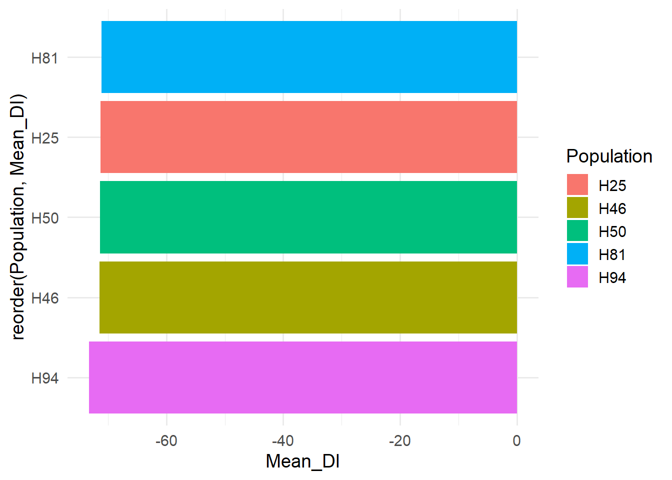

top5 <- selected$GEN
DesireIndex_pop <- DesireIndex_pop %>%
  dplyr::mutate(
    Elite = ifelse(GEN %in% top5, "Selected", "Not Selected"))

library(ggplot2)
library(ggrepel)

DGIPLOT = ggplot(
  DesireIndex_pop,
  aes(
    x = Population,
    y = DesireIndex
  )
) +

  geom_boxplot(
    aes(fill = Cross),
    width = 0.9,
    alpha = 0.13,
    linewidth = 0.5,
    outlier.shape = NA
  ) +

  # Points
  geom_jitter(
    aes(
      color = Elite,
      shape = Elite),
    width = 0.15,
    size = 3,
    alpha = 0.8) +
  # Labels for non-selected lines
  geom_text_repel(
    data = subset(DesireIndex_pop, Elite == "Not Selected"),
    aes(label = GEN),
    size = 4,
    fontface = "bold",
    alpha = 0.75,
    color = "black",
    max.overlaps = Inf,
    box.padding = 0,
    point.padding = 1,
    segment.alpha = 0) +
  # Labels for selected lines
  geom_text_repel(
    data = subset(DesireIndex_pop, Elite == "Selected"),
    aes(label = GEN),
    size = 6,
    fontface = "bold",
    alpha = 0.75,
    color = "purple",
    max.overlaps = Inf,
    box.padding = 0.3,
    point.padding = 1,
    segment.alpha = 0) +
  scale_shape_manual(
    values = c(
      "Not Selected" = 20,
      "Selected" = 20
    ),
  guide = "none") +
  scale_color_manual(
    values = c(
      "Not Selected" = "black",
      "Selected" = "purple"),
  guide = "none")  +
  scale_fill_manual(
  values = c(
    "G25236 × BGP UFPI 628"       = "#FF5E66",
    "UC HASKELL × BGP UFPI 728"   = "#FFF75E",
    "BGP UFPI 728 × BGP UFPI 628" = "#5EB7FF",
    "BGP UFPI 628 × UC 92"        = "#66FF5E",
    "BGP UFPI 728 × UC 92"        = "#FF5EB7"
  ),
  name = "Cross" )+
  labs(
    x = "Population",
    y = "Desire Gain Index",
    color = NULL,
    shape = NULL) +
  theme_classic(base_size = 12) +
  theme(
    panel.grid = element_blank(),
    axis.line = element_line(
      colour = "black",
      linewidth = 1),
    axis.title.x = element_text(
      face = "bold",
      size = 14),
    axis.title.y = element_text(
      face = "bold",
      size = 14),
    axis.text.x = element_text(
      face = "bold",
      size = 12),
    axis.text.y = element_text(
      face = "bold",
      size = 12),
    legend.text = element_text(
      face = "bold",
      size = 6),
    legend.position = c(0.55, 0.18)
  )
DGIPLOT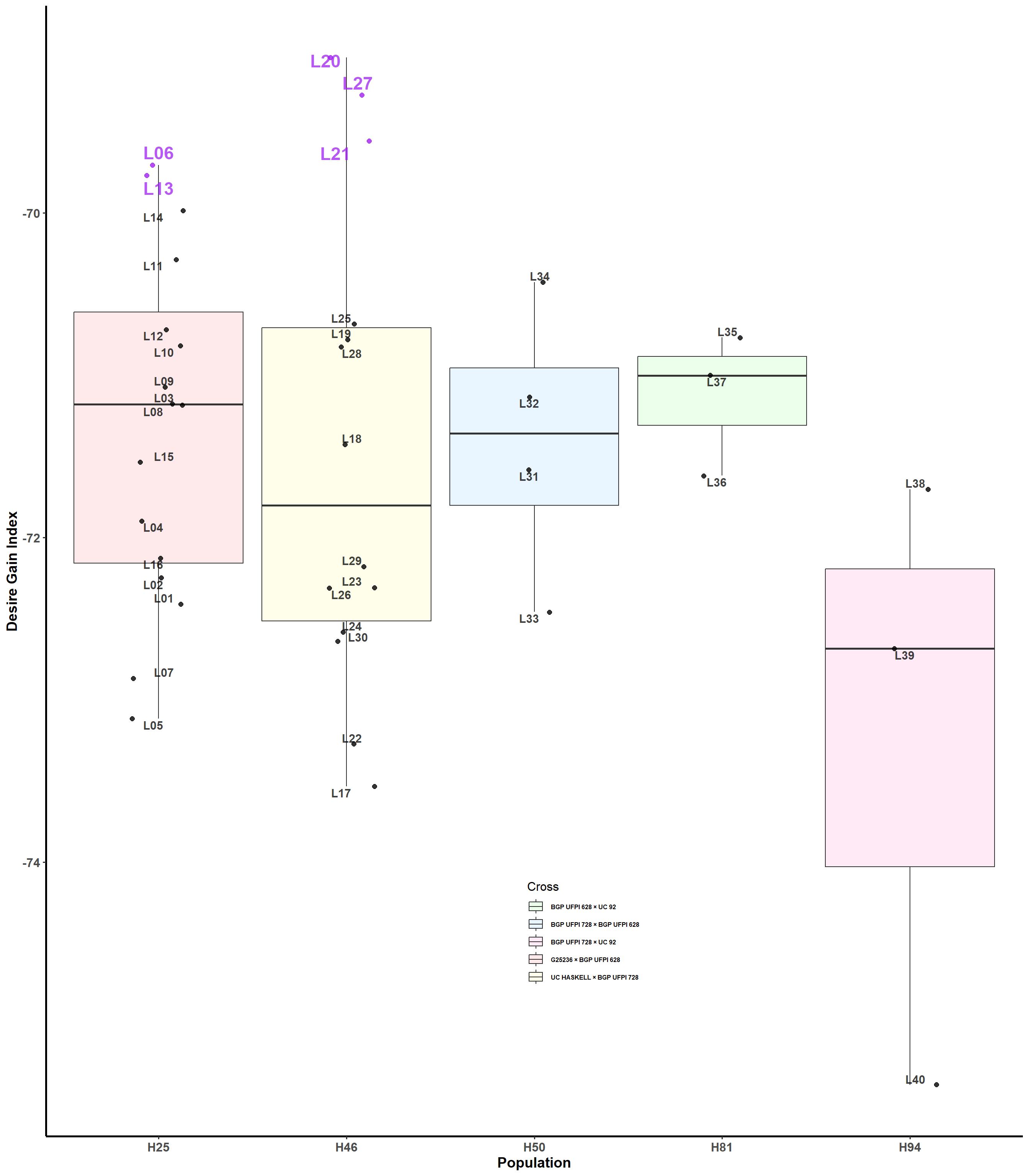

Genotype by trait (GT) biplot

library(ggplot2)
gtb1 <- gtb(
  LB,
  GEN,
  resp = c(NDF, NDM, PH, PN, GY, OHSW))
gtb1plot <- plot(
  gtb1,
  col.env = "orange",
  col.gen = "purple",
  size.text.gen = 4,
  size.text.env = 4,
  repel = TRUE,
  repulsion = 4,
  col.line = "darkorange",
  print.sub = FALSE,
  plot_theme = theme_bw(base_size = 14) +
    theme(
      plot.title = element_blank(),
      plot.subtitle = element_blank(),
      panel.grid = element_blank(),
      legend.position = c(0.85, 0.2),
      legend.title = element_blank()))
gtb1plot$layers[[5]]$aes_params$alpha <- 0.4
gtb1plot$layers[[5]]$aes_params$size  <- 3
gtb1plot <- gtb1plot +
  annotate(
    "text",
    x = Inf,
    y = -Inf,
    label = "Scaling = 1, Centering = 2, SVP = 2",
    hjust = 1.1,
    vjust = -0.8,
    fontface = "bold",
    size = 3
  )

Arrange

gt_desired_panel <- ggarrange(gtb1plot, desiredgainplot,
  ncol = 2,
  common.legend = F, legend = "bottom",
  labels = c("A","B"),
  font.label = list(size = 10, face = "bold"), 
  align = "hv",
  hjust = -0.5,
  vjust = 1.5
)
gt_desired_panel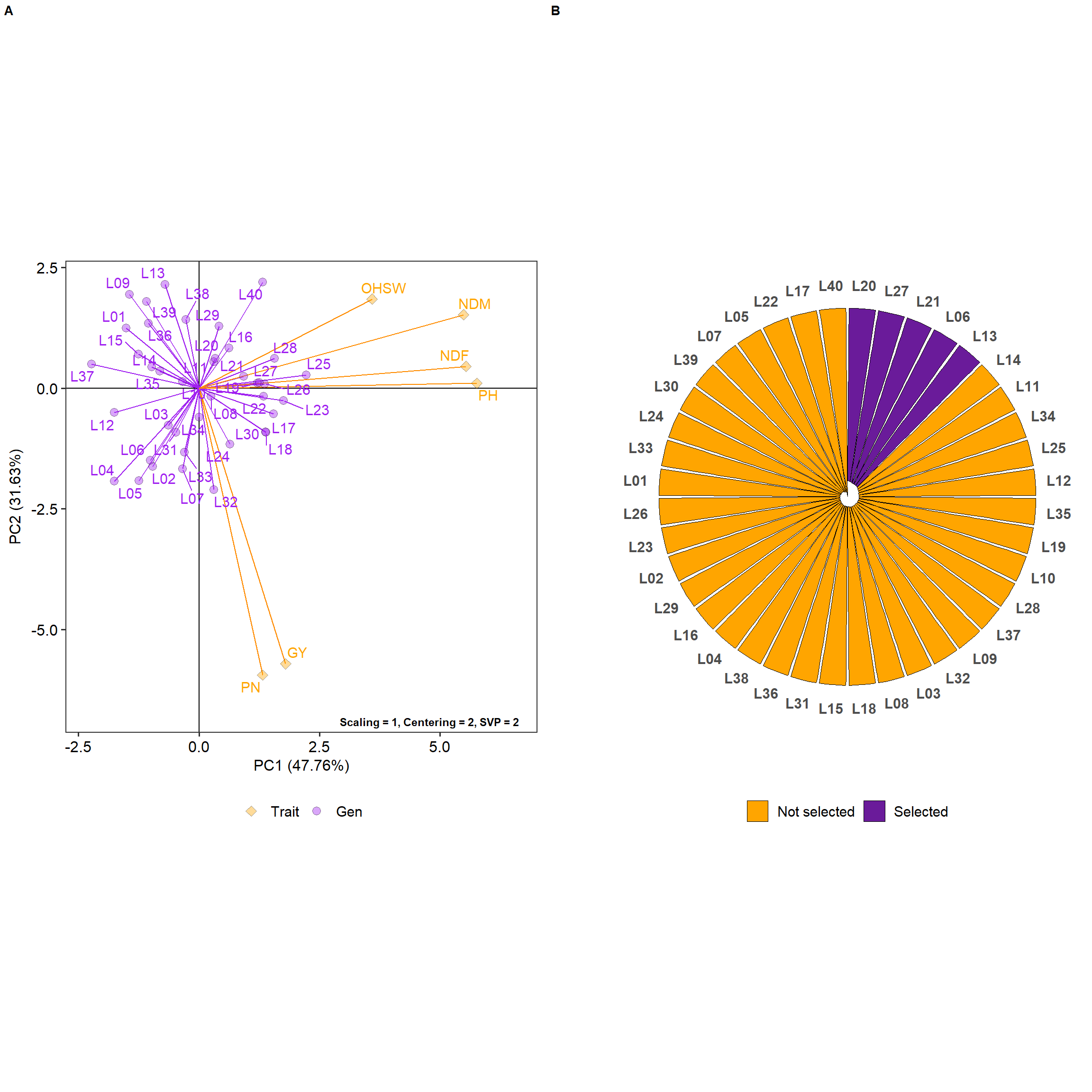

ggsave("gt_desired_panel_LB.pdf", plot = gt_desired_panel, dpi = 600)

Selection shift plot

library(dplyr)
library(tidyr)
library(ggplot2)
library(ggridges)
trait_names <- c(
  GY_BLUP   = "GY (kg/ha)",
  OHSW_BLUP = "OHSW (g)",
  PN_BLUP  = "PN (Number)",
  PH_BLUP  = "PH (cm)",
  NDF_BLUP   = "NDF (days)",
  NDM_BLUP   = "NDM (days)")
df_long <- bind_rows(
  lapply(names(BLUPgen), function(tr) {
  
    BLUPgen[[tr]] %>%
      dplyr::mutate(
        Trait  = trait_names[[tr]],
        Status = ifelse(
          GEN %in% selected$GEN,
          "Selected",
          "Not Selected")) %>%
      dplyr::select(
        GEN,
        Trait,
        Status,
        Predicted)
  }))

library(ggplot2)
library(dplyr)
library()
df_long$Trait <- factor(
  df_long$Trait,
  levels = c(
    "GY (kg/ha)",
    "OHSW (g)",
    "PN (Number)",
    "PH (cm)",
    "NDF (days)",
    "NDM (days)"
  )
)
# Cullis heritability table
h2_df <- data.frame(
  Trait = c(
    "GY (kg/ha)",
    "OHSW (g)",
    "PN (Number)",
    "PH (cm)",
    "NDF (days)",
    "NDM (days)"
  ),
  H2 = c(
    0.303,
    0.754,
    0.281,
    0.528,
    0.752,
    0.403))

h2_df$Trait <- factor(
  h2_df$Trait,
  levels = levels(df_long$Trait))
# Plot
SelectionShiftPlot <- ggplot(
  df_long,
  aes(
    x = Status,
    y = Predicted,
    fill = Status)) +
  # Violin
  geom_violin(
    alpha = 0.25,
    color = "black",
    linewidth = 1.2,
    trim = FALSE) +
  # Boxplot
  geom_boxplot(
    width = 0.12,
    alpha = 0.3,
    linewidth = 0.6,
    outlier.shape = NA) +
  # Individual genotypes
  geom_jitter(
    width = 0.08,
    size = 1.5,
    alpha = 0.45,
    color = "black") +
  # Mean
  stat_summary(
    fun = mean,
    geom = "point",
    shape = 23,
    size = 3,
    fill = "white",
    color = "black",
    stroke = 1) +
  facet_wrap(
    ~Trait,
    scales = "free_y",
    ncol = 2, nrow = 3) +
  # Heritability annotation
  geom_text(
    data = h2_df,
    aes(
      x = 1.5,
      y = Inf,
      label = paste0(
        "H[Cullis]^2==",
        sprintf("%.3f", H2))),
    inherit.aes = FALSE,
    parse = TRUE,
    fontface = "bold",
    size = 4,
    vjust = 1.5) +
  scale_fill_manual(
    values = c(
      "Not Selected" = "orange",
      "Selected" = "purple")) +
  labs(
    x = NULL,
    y = "Predicted",
    fill = NULL) +
  ggdist::theme_ggdist(base_size = 14) +
  theme(
    panel.grid = element_blank(),
    strip.background = element_rect(
      fill = "grey95",
      colour = "black",
      linewidth = 0.5),
    strip.text = element_text(
      face = "bold",
      size = 12),
    axis.title.y = element_text(
      face = "bold",
      size = 13),
    axis.text.x = element_text(
      face = "bold",
      size = 11),
    axis.text.y = element_text(
      face = "bold",
      size = 11),
    legend.position = "none",
    legend.text = element_text(
      face = "bold",
      size = 11),
    panel.spacing = unit(1.2, "lines"))
SelectionShiftPlot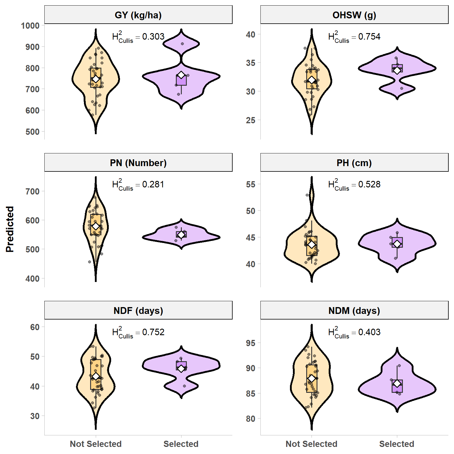

ggsave("SelectionShiftPlot.pdf", plot = SelectionShiftPlot, 
       width = 8,
       height = 8,
       dpi = 600)

Density plot

ggsave(plot = densplot, "densplot.pdf", width = 14, height = 8, dpi = 600)

Environmental Similarity

library(EnvRtype)
library(terra)
library(raster)
library(dplyr)
library(ggplot2)
library(reshape2)

# ENVIRONMENTS
env.i <- c(
  "Piracicaba (SP)",
  "Teresina (PI)",
  "Tianguá (CE)"
)

lat <- c(-22.708333, -5.093889, -3.732222)
lon <- c(-47.636667, -42.784722, -41.012222)

plant.date <- c("2024-12-19", "2023-03-14", "2023-02-14")
harv.date  <- c("2025-04-15", "2023-07-14", "2023-06-14")

# WEATHER DATA
df.clim <- get_weather(
  env.id = env.i,
  lat = lat,
  lon = lon,
  start.day = plant.date,
  end.day = harv.date
)

# CLIMATE COVARIATES
var.clim <- c("T2M", "VPD", "PRECTOT", "GWETTOP")

df.clim$DATE <- as.Date(as.character(df.clim$YYYYMMDD), format = "%Y%m%d")
df.clim$YEAR <- as.numeric(format(df.clim$DATE, "%Y"))
df.clim$MM   <- as.numeric(format(df.clim$DATE, "%m"))
df.clim$DD   <- as.numeric(format(df.clim$DATE, "%d"))

EC <- W_matrix(
  env.data = df.clim,
  env.id = "env",
  var.id = var.clim,
  statistic = "mean"
)

EC <- data.frame(env = rownames(EC), EC, row.names = NULL)

# SOIL RASTER
soilraster <- raster(
  "C:/Users/joaop/Documents/GitHub/Kenya Maps/KenyaMaps/Soil_Raster/hwsd_domi.tif"
)

coords <- data.frame(env = env.i, lon = lon, lat = lat)

soil_values <- extract(soilraster, coords[, c("lon", "lat")])

soil_class <- data.frame(env = env.i, soil_class = soil_values)

soil_class_names <- data.frame(
  soil_class = c(1, 10),
  class_name = c("Lixisol", "Regosol")
)

soil_class <- left_join(soil_class, soil_class_names, by = "soil_class")

# MERGE CLIMATE + SOIL
EC_soil <- left_join(
  EC,
  soil_class[, c("env", "class_name")],
  by = "env"
)

# DUMMY VARIABLES (FIXED)
soil_dummy <- model.matrix(~ class_name - 1, data = EC_soil)
soil_dummy <- as.data.frame(soil_dummy)

# FINAL MATRIX
EC_final <- cbind(
  EC_soil %>% dplyr::select(-class_name),
  soil_dummy
)

EC_numeric <- EC_final %>% dplyr::select(where(is.numeric))
EC_numeric <- as.matrix(EC_numeric)

rownames(EC_numeric) <- EC_final$env

# IMPUTE NA
for (i in 1:ncol(EC_numeric)) {
  EC_numeric[is.na(EC_numeric[, i]), i] <- mean(EC_numeric[, i], na.rm = TRUE)
}

# ENVIRONMENTAL KERNEL
K_E <- env_kernel(env.data = EC_numeric)[[2]]

# HEATMAP DATA
K_df <- melt(K_E)

colnames(K_df) <- c("Env1", "Env2", "Similarity")

K_df <- K_df %>%
  dplyr::mutate(
    Env1 = factor(Env1, levels = rownames(K_E)),
    Env2 = factor(Env2, levels = colnames(K_E))
  ) %>%
  filter(as.numeric(Env1) >= as.numeric(Env2))

# PLOT
envsim <- ggplot(K_df, aes(Env1, Env2, fill = Similarity)) +

  geom_tile(color = "white", linewidth = 0.5) +

  scale_fill_gradientn(
    colors = c("purple", "#b2abd2", "#f7f7f7", "#fdb863", "orange"),
    name = "Environmental Similarity"
  ) +

  coord_equal() +

  theme_minimal(base_size = 16) +

  theme(
    panel.grid = element_blank(),

    axis.text.x = element_text(face = "bold", size = 12),
    axis.text.y = element_text(face = "bold", size = 12),

    axis.title = element_blank(),

    plot.title = element_text(
      face = "bold",
      hjust = 0.5,
      size = 18
    ),

    legend.position = "bottom",

    legend.title = element_text(face = "bold", size = 12),
    legend.text = element_text(face = "bold", size = 10)
  )

library(igraph)
library(ggraph)
library(ggplot2)
env_df <- data.frame(
  env = c(
    "Piracicaba",
    "Teresina",
    "Tianguá"
  ),
  x = c(0, 1, 0.5),
  y = c(0, 0, 0.9)
)

envsim2 = ggplot(env_df, aes(x, y)) +

  # triangle
  geom_polygon(
    fill = "#F7F7F7",
    color = "grey40",
    linewidth = 1.2,
    alpha = 0.5
  ) +

  # environment points
  geom_point(
    aes(fill = env),
    shape = 21,
    size = 20,
    color = "black",
    stroke = 0
  ) +

  # environment labels
  geom_text(
    aes(label = env),
    fontface = "bold",
    size = 5,
    nudge_y = 0,
    nudge_x = 0
  ) +

  # similarity values
  annotate(
    "text",
    x = 0.5,
    y = 0.05,
    label = round(K_E[1,2], 2),
    size = 5,
    fontface = "bold"
  ) +

  annotate(
    "text",
    x = 0.25,
    y = 0.45,
    label = round(K_E[1,3], 2),
    size = 5,
    fontface = "bold"
  ) +

  annotate(
    "text",
    x = 0.75,
    y = 0.45,
    label = round(K_E[2,3], 2),
    size = 5,
    fontface = "bold") +

  scale_fill_manual(
    values = c(
      "Piracicaba" = "purple",
      "Teresina"   = "orange",
      "Tianguá"    = "lightpink")) +

  coord_equal() +
  theme_void() +
  theme(
    legend.position = "none"
  )
envsim2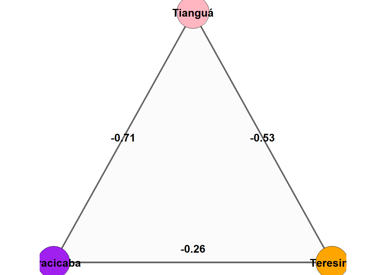

ggsave("envsim2.pdf", plot = envsim2, 
       width = 8,
       height = 8,
       dpi = 600)